Update 25.3.2021: I haven't ended up using PySpark as much as I might have hoped or expected, but I think this post has some interesting ideas in it all the same!

Introduction

Recently, I published the paper Revisiting the envelope approximation: gravitational waves from bubble collisions. This work compares two methods for computing the gravitational wave power spectrum from colliding bubbles from a phase transition in the early universe. It turned out to be an ideal example of a physics simulation in which the MapReduce algorithm can be applied.

Physics background and motivation

Normally, when I am doing numerical simulations of physics the system can be treated with domain decomposition methods - 3D and 4D lattice Monte Carlo simulations, and real-time simulations of physics in the early universe usually involve scalar fields \(\Phi(\mathbf{x})\), gauge fields, represented by parallel transporters (mini-Wilson lines) \(U_i(\mathbf{x})\) and also fermions \(\Psi(\mathbf{x})\). Normally, these fields exist everywhere in space and time; when doing a simulation they exist only inside our box (3D or 4D euclidean) and only on discrete points (or parallel transporters between those points). If a classical field theory, the box represents a state at a given time \(t\) and is evolved to the next timestep \(t+\delta t\) by some symplectic method. For quantum field theories, the box represents a configuration sampled from the Euclidean field theory with weight \(e^{-S[\Phi]}\). Parallelising these simulations means dividing the box into smaller boxes and sharing those out between different nodes, exchanging information every timestep (or Monte Carlo update) about the boundaries of each smaller box.

For simulating a first order phase transition, one can use a real-time lattice simulation. Several bubbles expand in a big box - but the number of points the box can contain is limited: either your computer will run out of memory, or you will run out of nodes to share the box across, or communicating the state of each smaller box to its neighbours will overwhelm the time you spend actually doing stuff. That gives you limited dynamic range

---

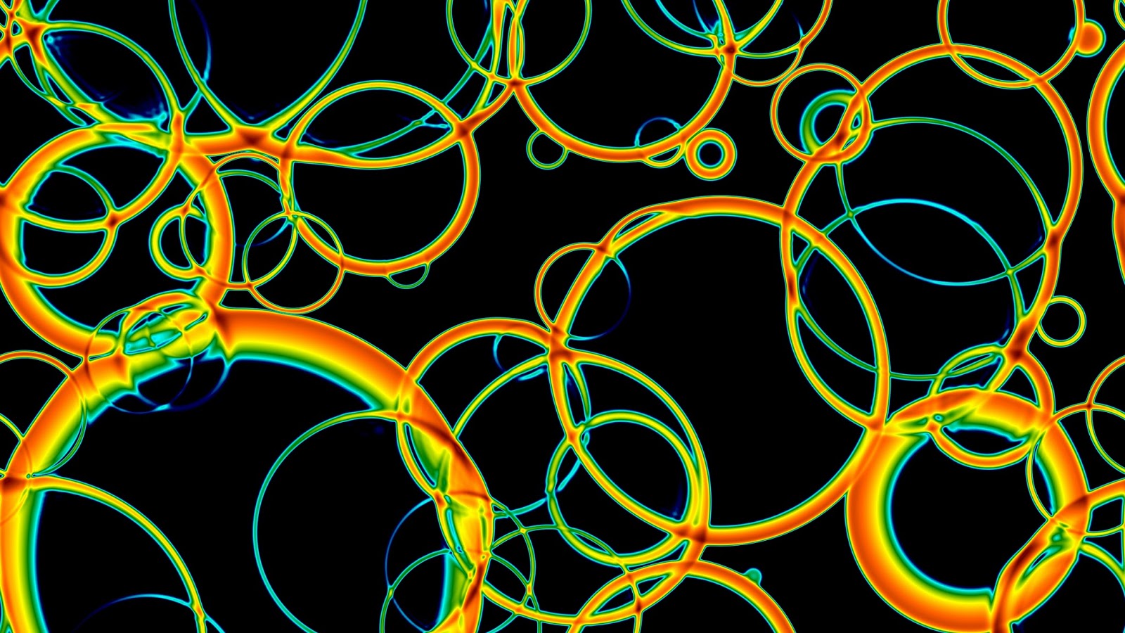Slice through a simulation of a first-order phase transition, such as that which might have happened when the Higgs became massive.

---

The envelope approximation is different

The envelope approximation is a way of computing the gravitational wave power spectrum from first-order phase transitions. To summarise briefly: in the Standard Model of particle physics, the Higgs particle got its mass in a gentle process, termed a crossover. However, we know the Standard Model is incomplete, and many extensions of it allow for situations where this happened in a much more violent manner. It is conceivable that bubbles of massive Higgs phase nucleated and grew, until the Higgs was massive in the whole universe. As the bubbles collided, they would produce a characteristic signature in gravitational waves, which we might be able to detect in the next couple of decades.

There's lots of jargon in there (and here is a recent summary on the state of the art, for the interested reader), but all you need to know is that, for a given simulation configuration the envelope approximation is a set of integrals that can be done in parallel (one per bubble), with the total gravitational wave power computed by summing the individual contributions from each integral.

Here is a perfect MapReduce problem: for each frequency \(\omega\) of the power spectrum we want to calculate map each thread to a different bubble \(n\), do the integrals for that bubble in splendid isolation, then reduce the total to compute the gravitational wave power \(\Omega_\text{gw}(\omega)\). The good news is a lot of the hard work is not strongly \(\omega\) dependent, so we can speed things up by giving each thread the same bubble \(n\) each time. This is what my code does, and it works pretty well. At the top level, it uses either MPI4py or PySpark. In fact, because this is such a natural MapReduce-style problem, the pyspark approach looks more natural! Below the top most layer of code, the actual calculations trivially parallelise and so there is no difference.

But what about fault tolerance?

Aha, this is the tricky one. Both [Py]Spark and MapReduce more generally, are claimed to have greater fault tolerance. Assuming the input data are available, each MapReduce step can be restarted easily enough - and indeed, in Spark this is automatic. However, the approach I outlined above does not benefit from this because the 'cached' data produced at one \(\omega\) is not stored as a Resilient Distributed Dataset, just a set of standard Python dictionaries. Restarting one of the threads will lose this cached data and slow things down.

And will you use MapReduce more in the future?

Absolutely. The diffusion equation example in Jonathan Dursi's post HPC is dying, and MPI is killing it was a revelation for me (code example is at the bottom). It's unlikely that performance of my simulation codes (in carefully written C, with MPI communication) would ever be reproduced using Spark with an interpreted language, but for a student wanting to do a small project and write their own code from scratch, I'd strongly recommend using it. Personally, I'll be sizing up every future project where I need to write a new code or heavily modify an existing one and asking myself "should I write this using a MapReduce-type approach?".

Afterword

I'm not finishing experimenting with my envelope approximation code. I plan to make it public on BitBucket soon (if you want to work with it right away, give me an email), and I also hope to modify the code so that the 'cache' data I mentioned to functions as an RDD. If and when these things happen, I'll update this blogpost.