Exploring gravitational waves from strong phase transitions

Exploring gravitational waves
from strong phase transitions

David J. Weir [they/he] - University of Helsinki
davidjamesweir@mementomori.social

This talk: saoghal.net/slides/vast2026

VAST 2026, Madrid, 23 October 2026

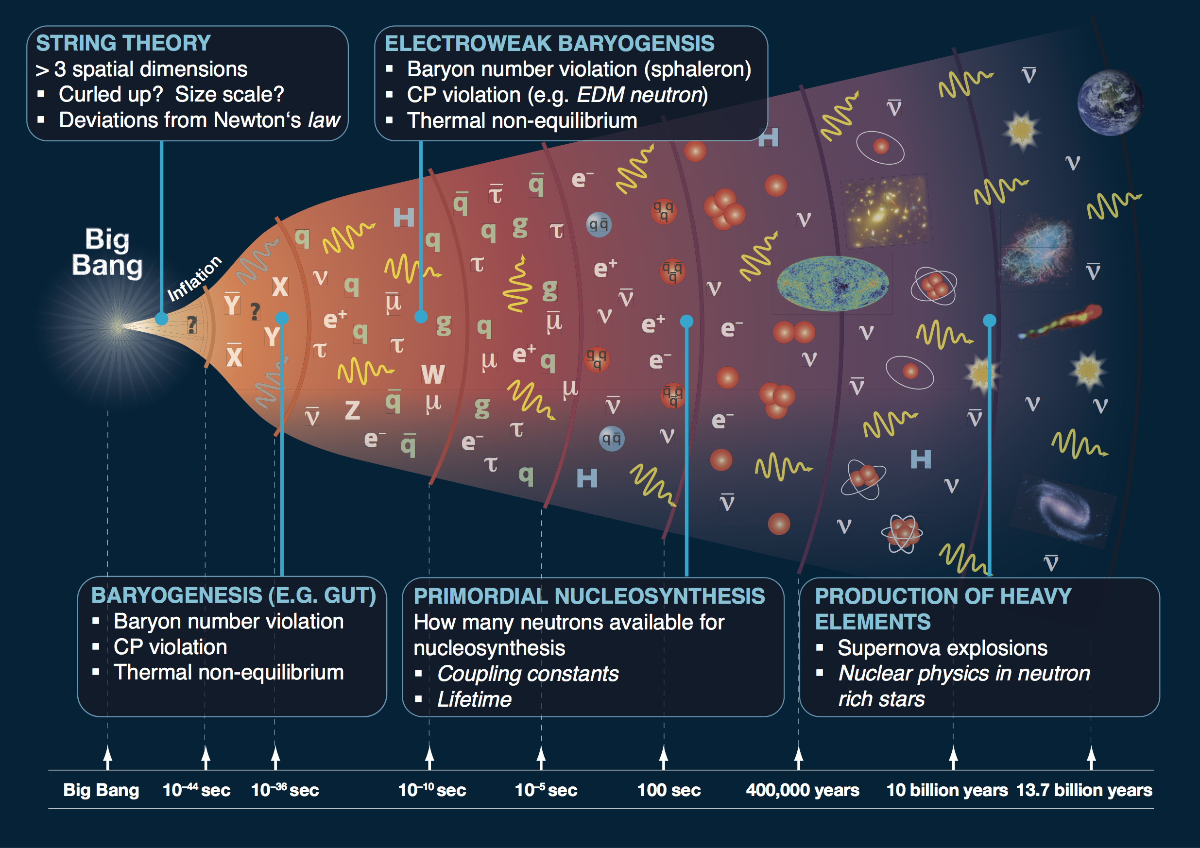
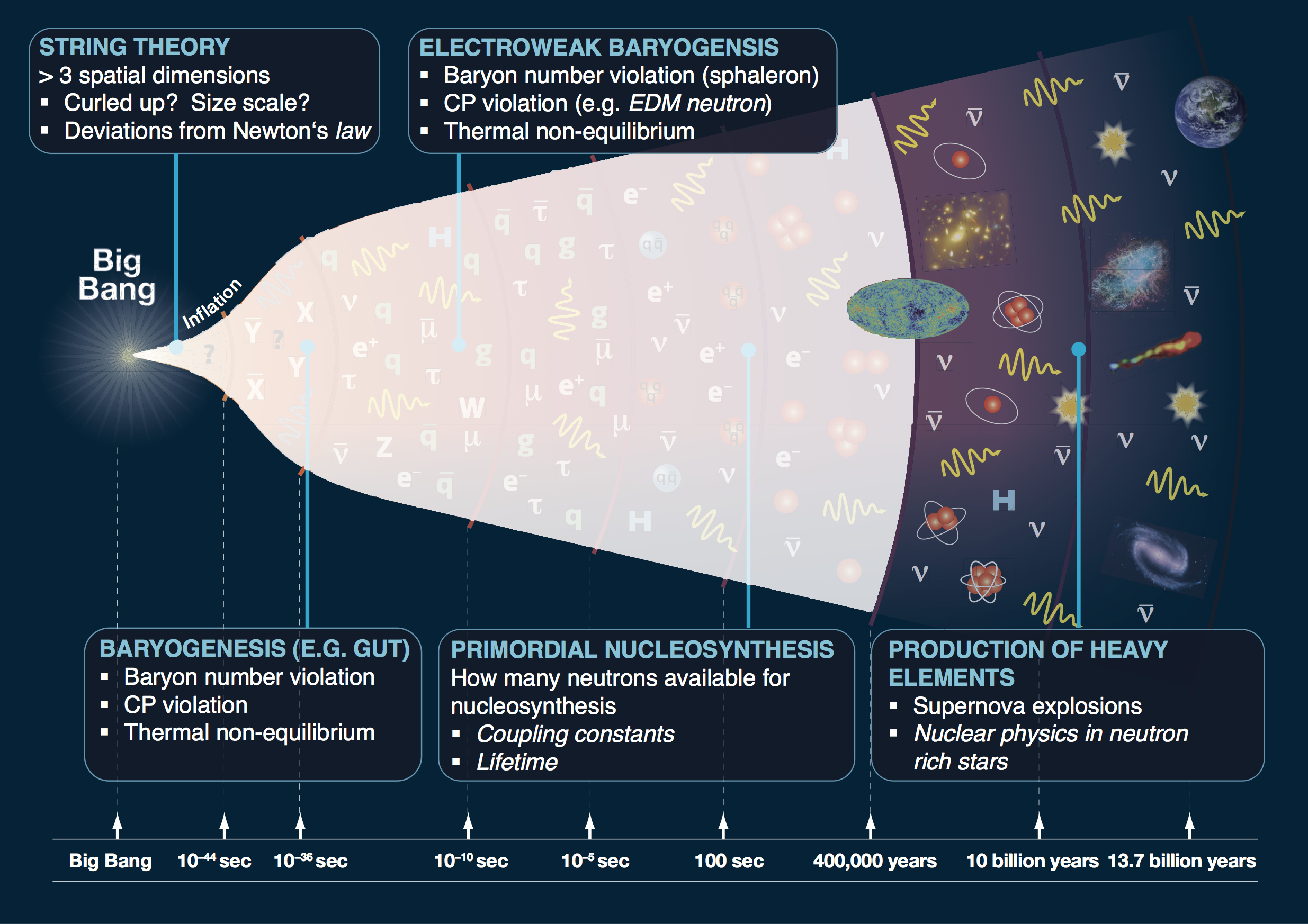
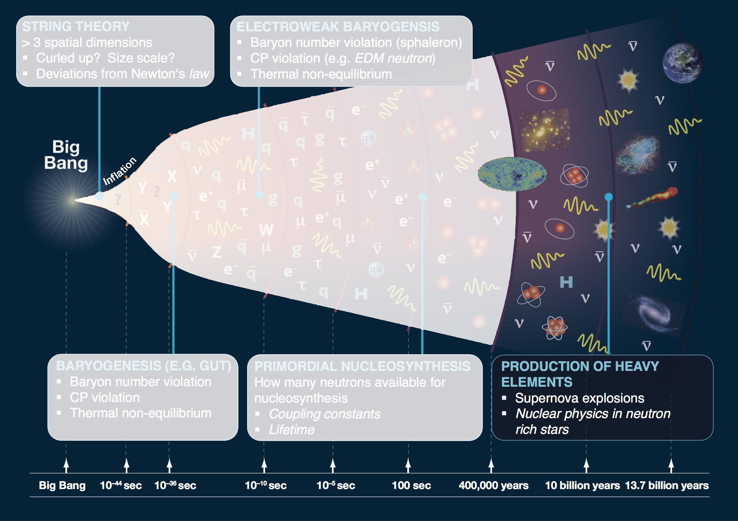
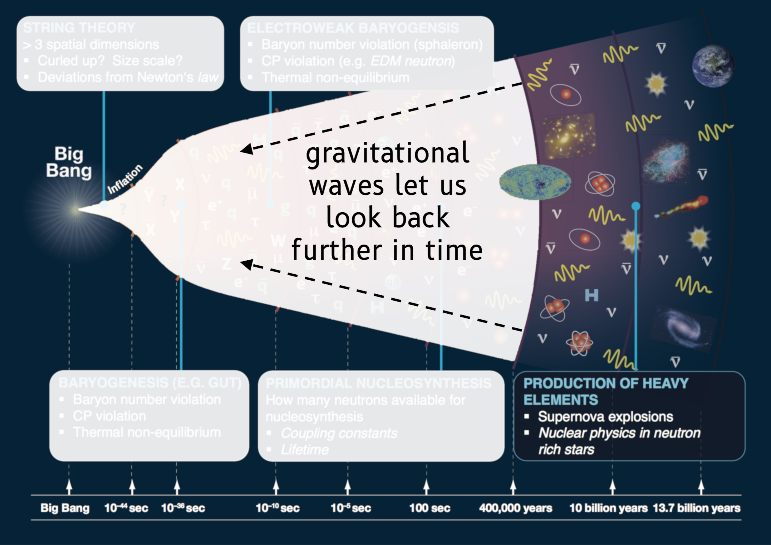
What happened in the early universe? before recombination? in dark sectors?

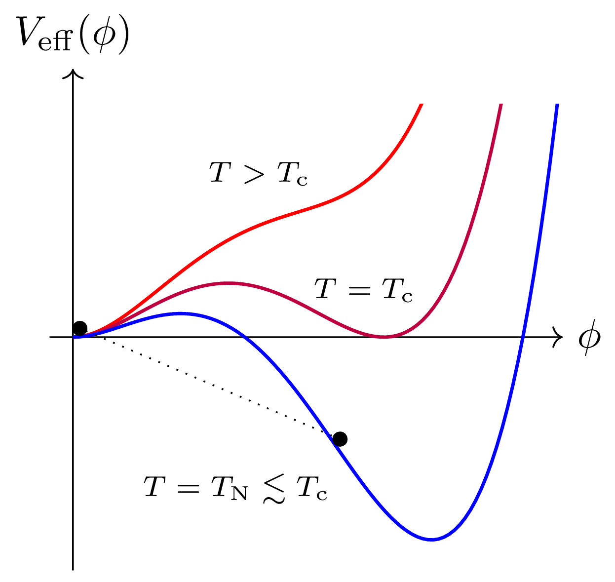
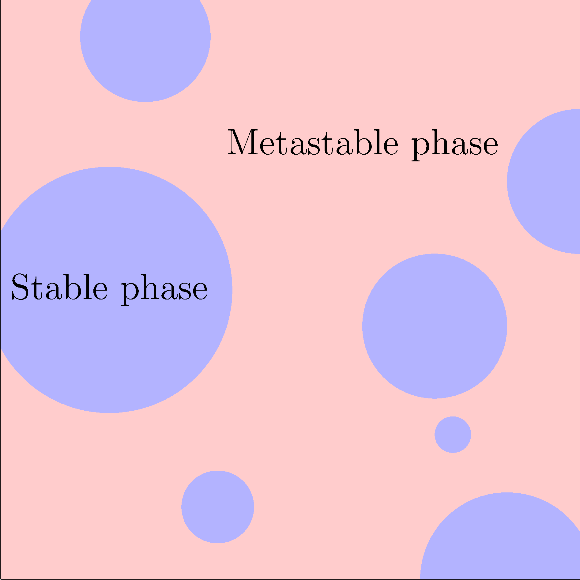
Credit: Stephan Paul, arXiv:1205.2451

First order phase transition

High temperatures: potential has one global minimum
Below $T_\mathrm{c}$, second minimum becomes global minimum
Nucleation temp. $T_\mathrm{n}$: ~ 1 bubble per causal volume
'Percolation' temp. $T_\mathrm{p}$: broken phase clusters join up

Summary: what happens?

Nucleation (temperatures $T_\mathrm{n}$→$T_\mathrm{p}$, duration $\beta^{-1}$)
Bubble walls expand in a plasma (at velocity $v_\mathrm{w}$)
Reaction fronts form around walls (with strength $\alpha$)

Detonations vs deflagrations

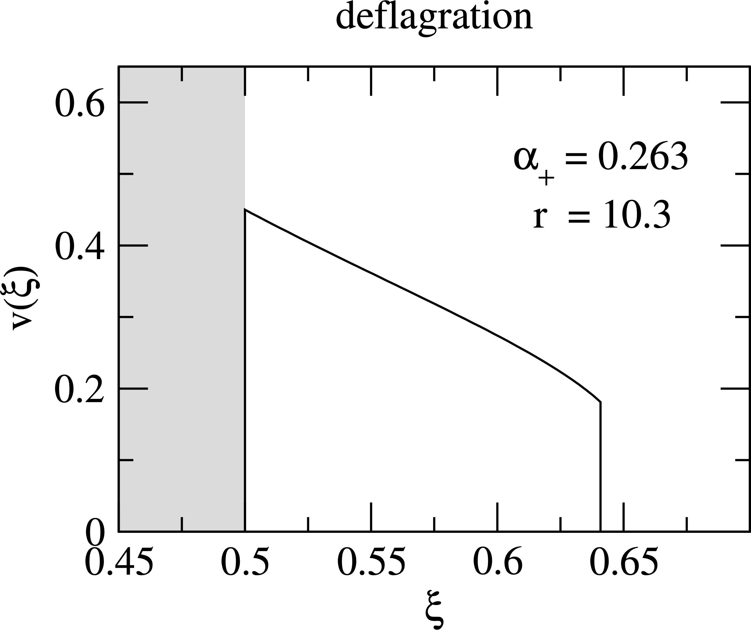
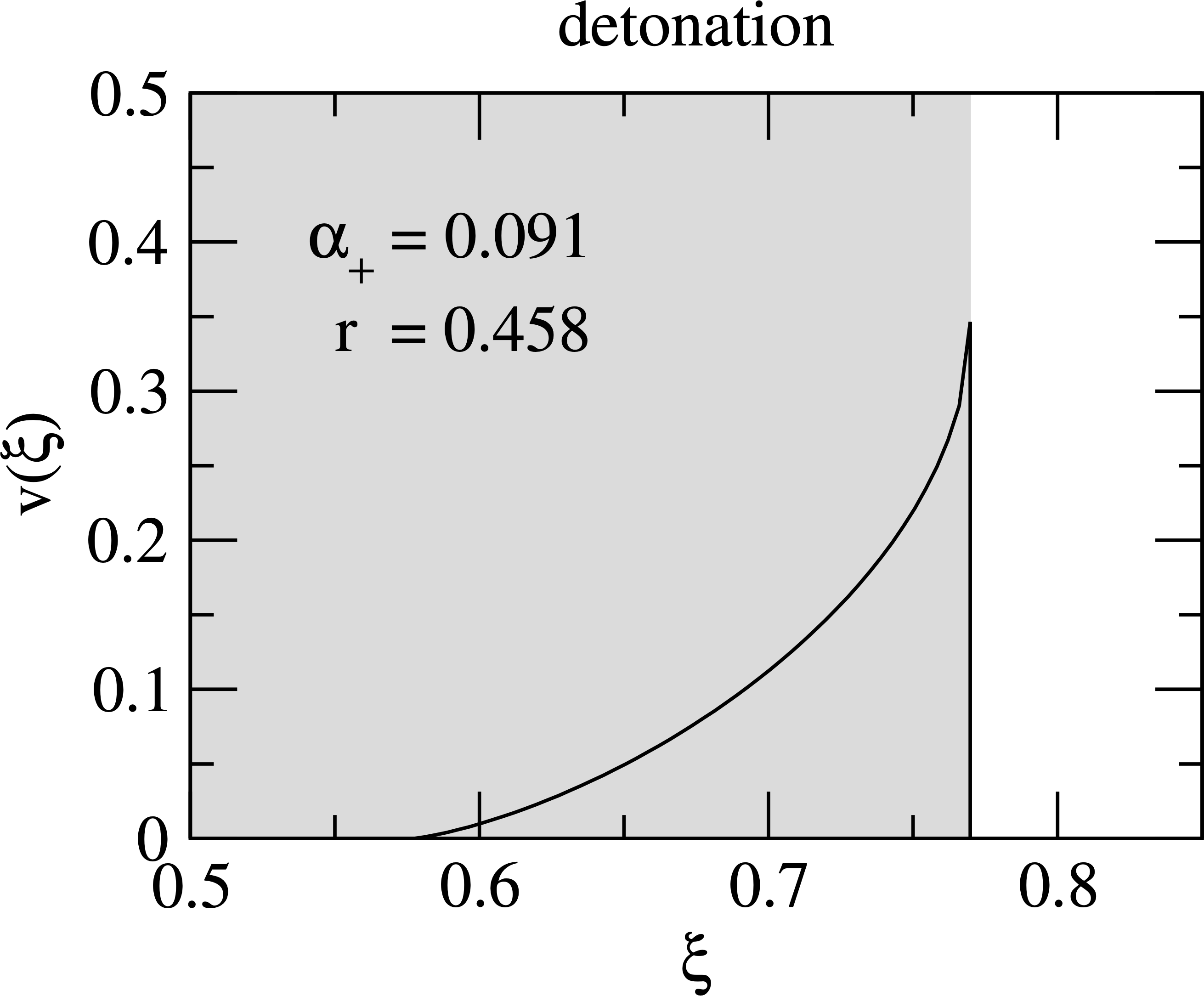
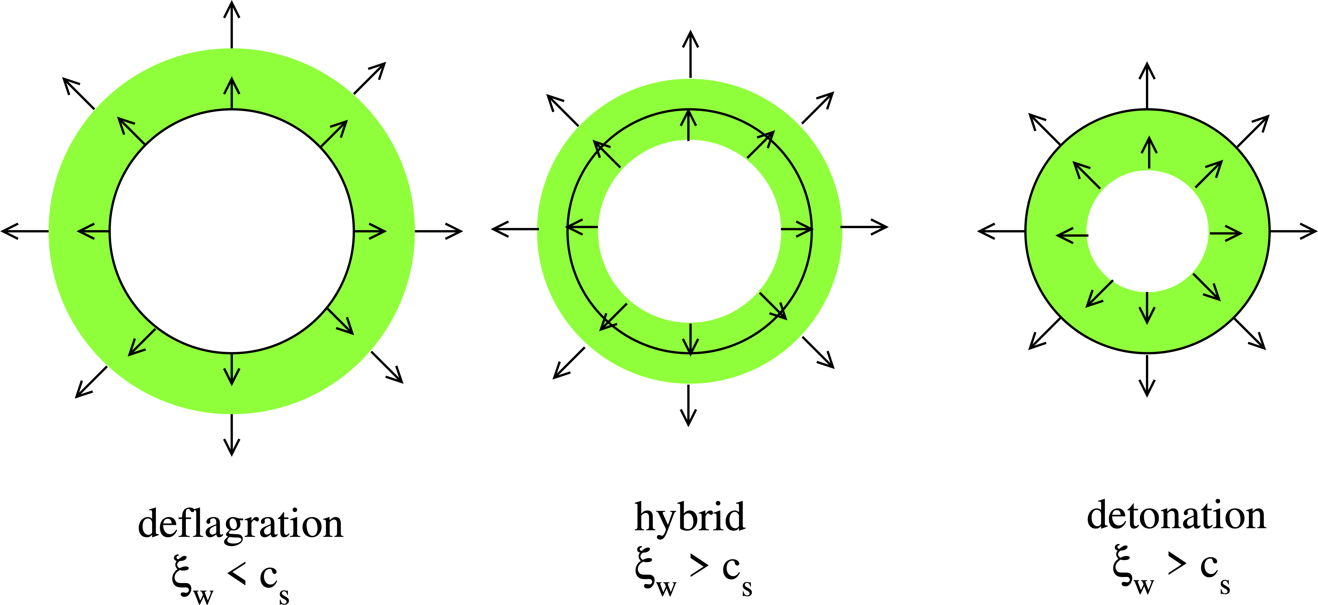
If the scalar field wall moves supersonically and the fluid enters the wall at rest, we have a detonation
If the scalar field wall moves subsonically and the fluid enters the wall at its maximum velocity, we have a deflagration
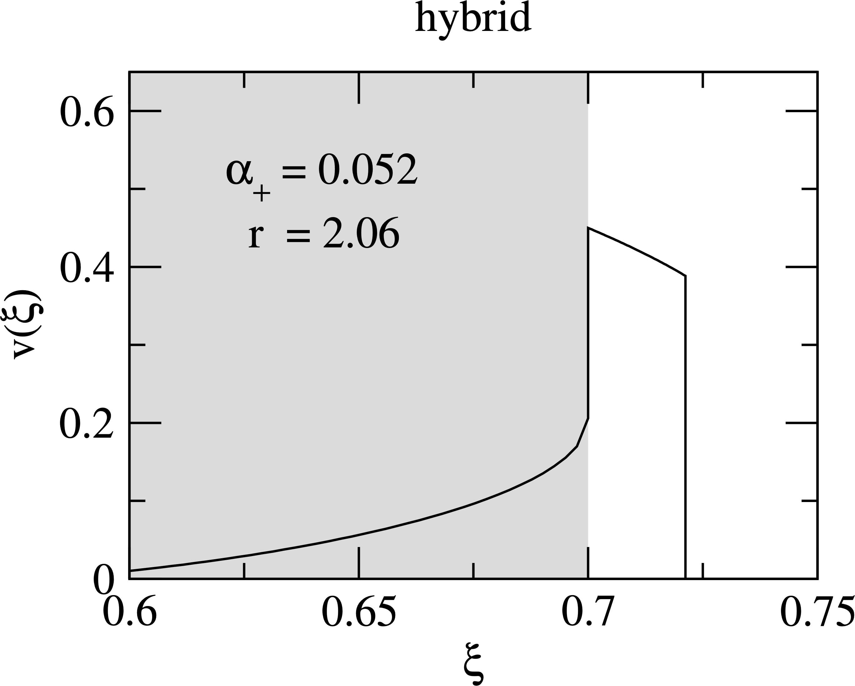
Can also get a hybrid where the wall moves supersonically but some fluid bunches up in front of it, like a deflagration

Detonations, hybrids, deflagrations

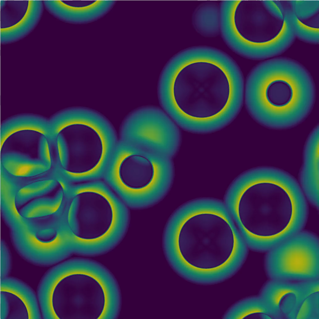
Source: Espinosa, Konstandin, No and Servant

OK, expanding bubbles associated with reaction fronts. Then what?

Bubbles (size $R_*$) + fronts collide GWs
Sound waves left behind, plasma 4-velocity $U$ GWs

System becomes 'turbulent'; KE starts to decay GWs
GW production saturates; Hubble damping

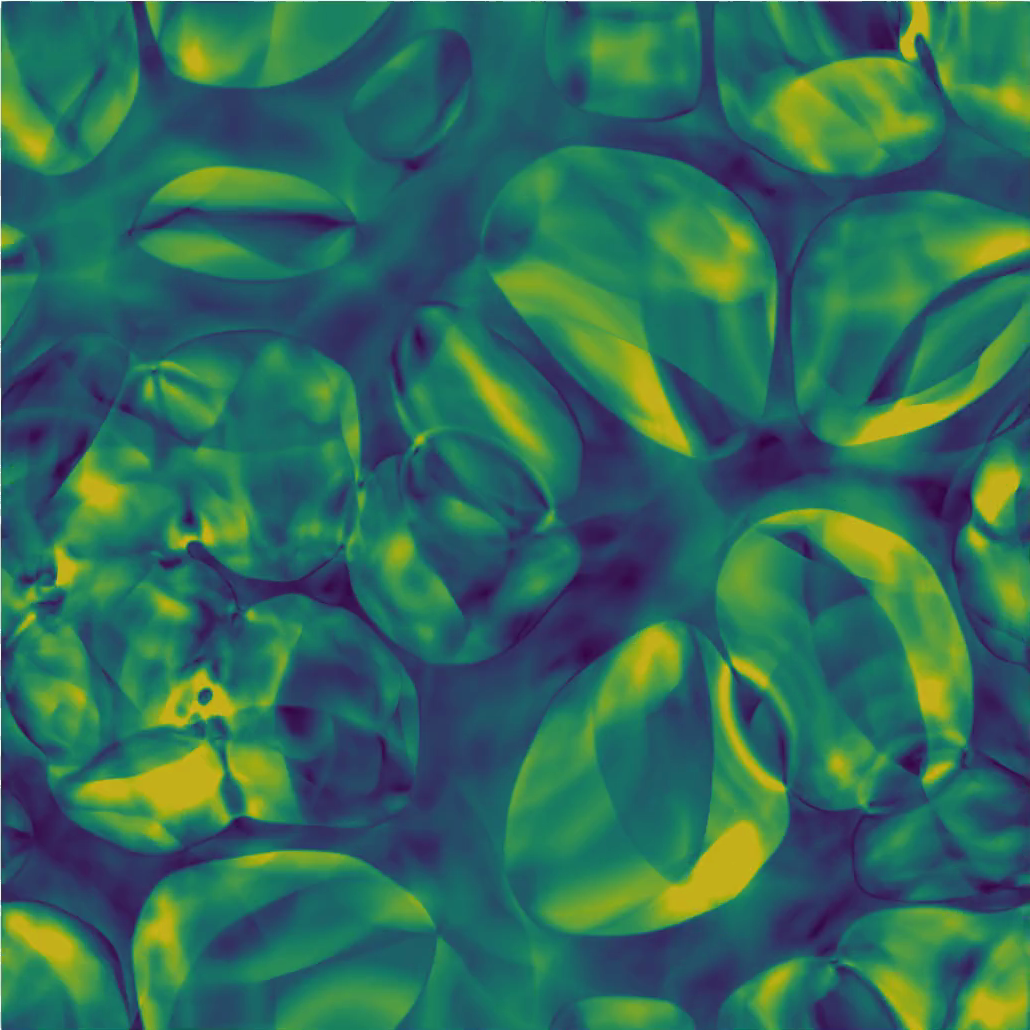
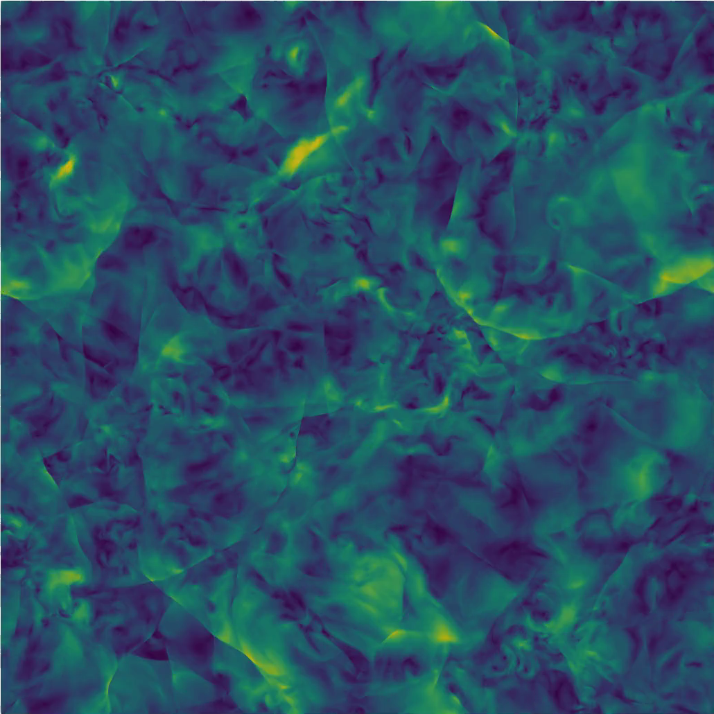
What is a strong phase transition?

Plasma velocities become relativistic
⇒ flows quickly become nonlinear
Nonlinearities include:
- shocks ➠ acoustic turbulence $t_{\mathrm{sh}} \sim R_* / U_{\parallel}$
- vortices ➠ [vortical] turbulence $t_{\mathrm{ed}} \sim R_* / U_{\perp}$
(in reality hard to separate into two types)
Transport of energy to small scales ⇒ KE decay
Typically strong means $\alpha$ 'large'
(maybe better to focus on what the flows look like)

Simulating a phase transition

Simulate scalar field $\phi$ and relativistic (ideal) fluid $u^\mu$, with $\eta$ friction term (e.g. our SCOTTS code)
- From $\partial_\mu T^{\mu\nu} = 0$: $$ \begin{align}\partial_\mu T^{\mu\nu}_\phi & = + \eta(\phi, v_\mathrm{w}) u^\mu \partial_\mu \phi \partial^\nu \phi \\ \partial_\mu T^{\mu\nu}_\mathrm{f} & = - \eta(\phi, v_\mathrm{w})u^\mu \partial_\mu \phi \partial^\nu \phi \end{align}$$
Either directly evolve metric perturbations sourced by the fluid $T_{ij}^\text{(f)} = w u_i u_j $ (from 0707.0839) ...
...or work with the velocity power spectrum.

Computing GWs in a simulation

Evolve harmonic-gauge, position-space wave equation: $ \nabla^2 h_{ij} (\mathbf{x},t) - \ddot{h}_{ij}(\mathbf{x},t) = 8 \pi G T_{ij}^\text{source}(\mathbf{x},t).$
Projection to TT-gauge requires expensive Fourier transform, so only project when measurement desired: $ h^{\text{TT}}_{ij}(\mathbf{k},t_\text{meas}) = \Lambda_{ij,lm}(\hat{\mathbf{k}}) h^{lm}(\mathbf{k},t) $
Measure energy density or power spectrum $$ \rho_\text{GW}(t_\text{meas}) = \frac{1}{32 \pi G} \left< \dot{h}_{ij}^\text{TT} \dot{h}_{ij}^\text{TT} \right> $$
Redshift to present day.

Other simulation codes/approaches

Other hydro codes (e.g. Pencil code) arXiv:1903.08585
- Can study nonlinear fluid motion after a transition
- Can't study physics of the transition itself
Higgsless code arXiv:2010.00971, arXiv:2209.04369, arXiv:2409.03651
- Bubble walls non-dynamical; swept through system
- Energy is injected at the bubble walls according to the (bag model) equation of state
- Cannot simulate slowing down of bubble walls
Other field+fluid codes include:
- Giblin and Mertens arXiv:1405.4005
- Cosmolattice arXiv:2607.27141

Strong simulation example

Created by José Correia for arXiv:2505.17824.

Sound shell model 1

$\alpha_n \ll 1$, $v_\mathrm{w} \ll 1$: sound waves are main GW source
- Neglect nonlinear interactions between bubbles etc.
- Also ignore later nonlinear motion in the fluid
  (i.e. shocks and turbulence)
Begin by obtaining the fluid velocity profile around the bubble wall, as a function of $\xi = r/t$,

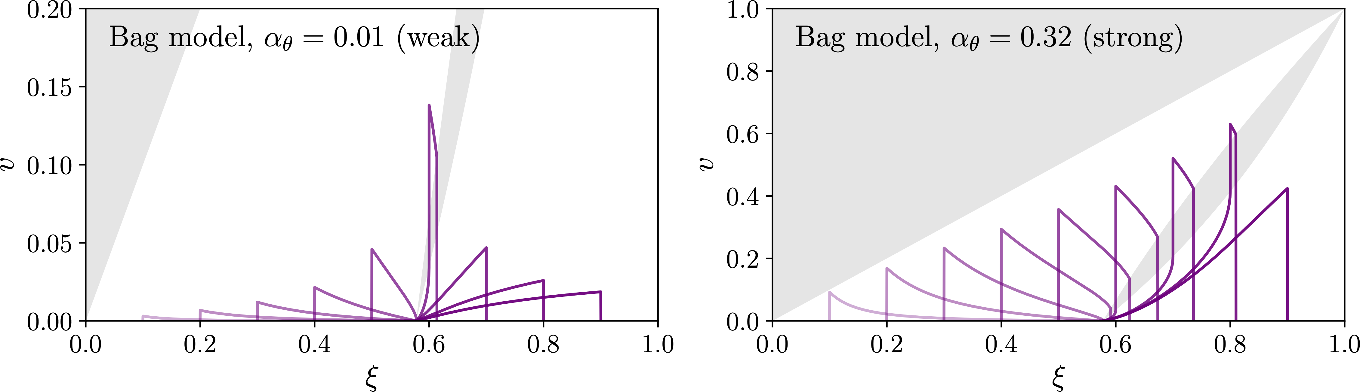
Sound shell model 2

arXiv:1608.04735; arXiv:1909.10040

Velocity power spectrum $P_v(f)$ from superposing random spherical shells with scaled profile $v(\xi)$
Convolve $P_v(f)$ with itself and integrate over time to get GW power spectrum

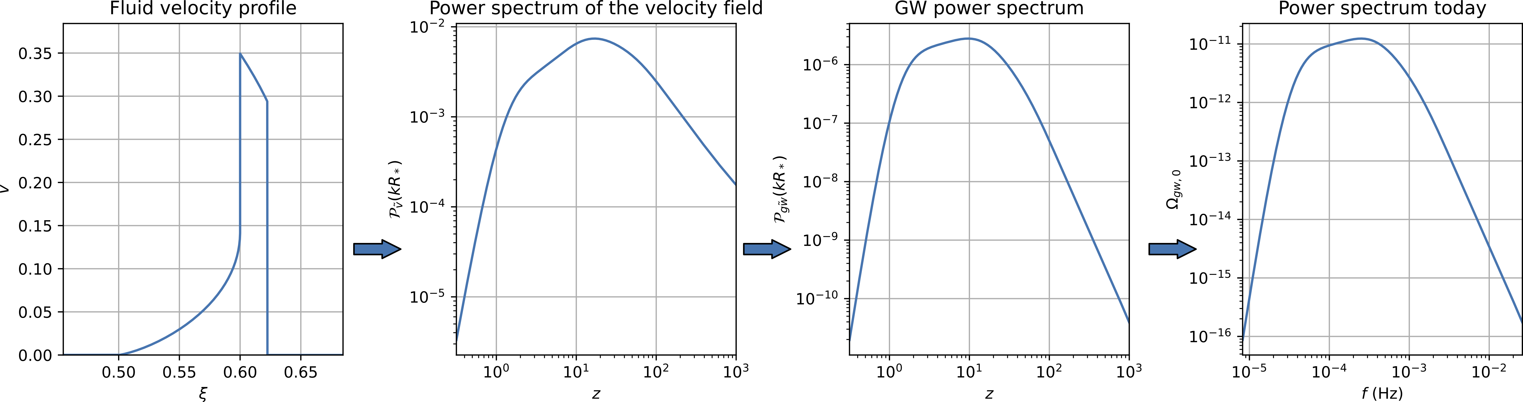
PTtools for fluid profiles/SSM

By Mika Mäki

pip-installable python package; Numba + JAX support
Everything (with sensible defaults) in 5+5 lines:


										from pttools.ssm import NucType
										from pttools.bubble import Bubble
										from pttools.models import BagModel
										from pttools.omgw0 import Spectrum
										import matplotlib.pyplot as plt
										
										model = BagModel(alpha_n_min=0.01)
										bubble = Bubble(model, v_wall=0.5, alpha_n=0.2)
										spectrum = Spectrum(bubble, nuc_type=NucType.EXPONENTIAL, r_star=0.1)
										spectrum_fig = spectrum.plot_multi()
										plt.savefig('spectrum_fig.pdf')

github.com/CFT-HY/pttools

Survey of ansätze 1

Single broken power law from 'CosWG20' arXiv:1910.13125: $$ \begin{multline} \Omega_\text{gw}(f) = \Omega_\text{gw, comm} \\ \times 0.687 \cdot \underbrace{\mathrm{min}(H_*\tau_\text{sh},1) (H_*R_*)}_{\text{life time} \times \text{coherence time}} C(f/f_\text{peak}) \end{multline} $$
where $\Omega_\text{gw, comm} = 3 \textcolor{red}{F_\text{gw,0}} \textcolor{blue}{K^2} \textcolor{purple}{\tilde{\Omega}_\text{gw}}$ combines:
dilution $\textcolor{red}{F_\text{gw,0}}$, PT efficiency $\textcolor{blue}{K^2}$, GW efficiency $\textcolor{purple}{\tilde{\Omega}_\text{gw}}$
Spectral shape $ C(s) = s^3 \left(\frac{7}{4 + 3 s^2}\right)^{\frac{7}{2}} $ i.e. $f^3 \to f^{-1}$
'Inspired by' simulations arXiv:1704.05871

Survey of ansätze 2

Double broken power law from 'GH21' arXiv:2106.05984: $$ C(s) = s^9 \left( \frac{1+ r_b^4}{r_b^4 + s^4}\right)^{\frac{9-b}{4}}\left( \frac{b + 4}{b + 4 -m + ms^2}\right)^{\frac{b+4}{2}} $$
$f^9 \to f^b \to f^{-4}$ with peaks at $s=1$ and $s=r_b$
$m$ chosen such that $C(1) = 1$ for $r_b < 1$
$r_b$ and $b$ chosen by fitting to SSM results
Different DBPL in arXiv:2403.03723 ('CosWG24')

How strong a phase transition do you need to see something at LISA?

(Assuming double broken power law ansatz) arXiv:2106.05984

$r_* = H_* R_*$ (ratio of bubble to Hubble)

SNR

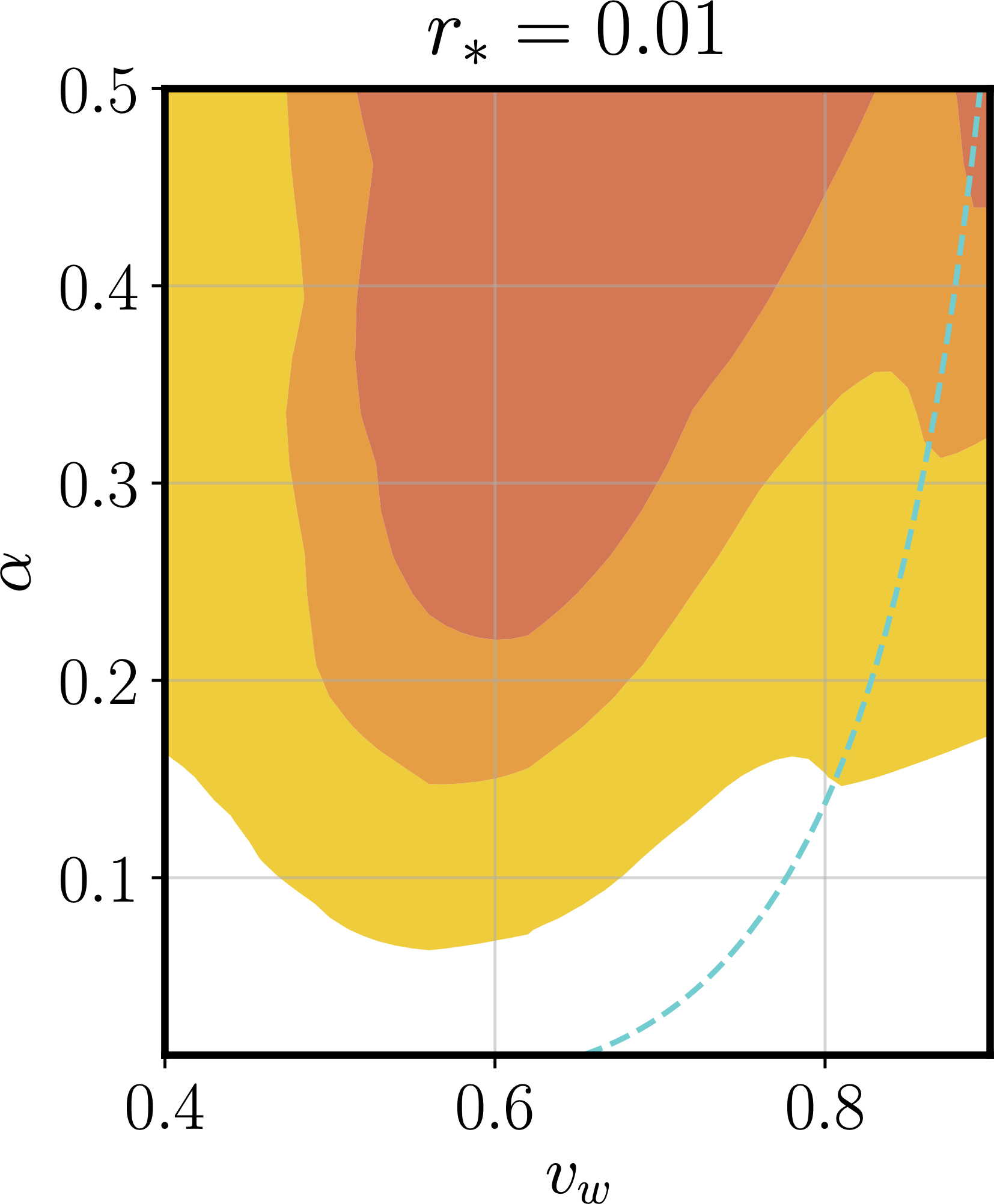
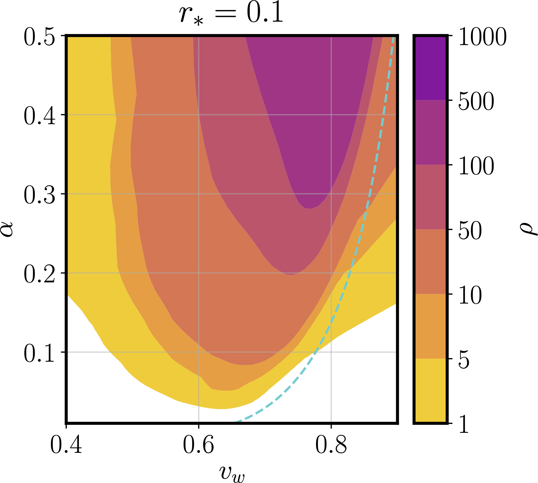
But: is a double broken power law valid when $\alpha$ is big?

Ansätze vs. simulation results 1

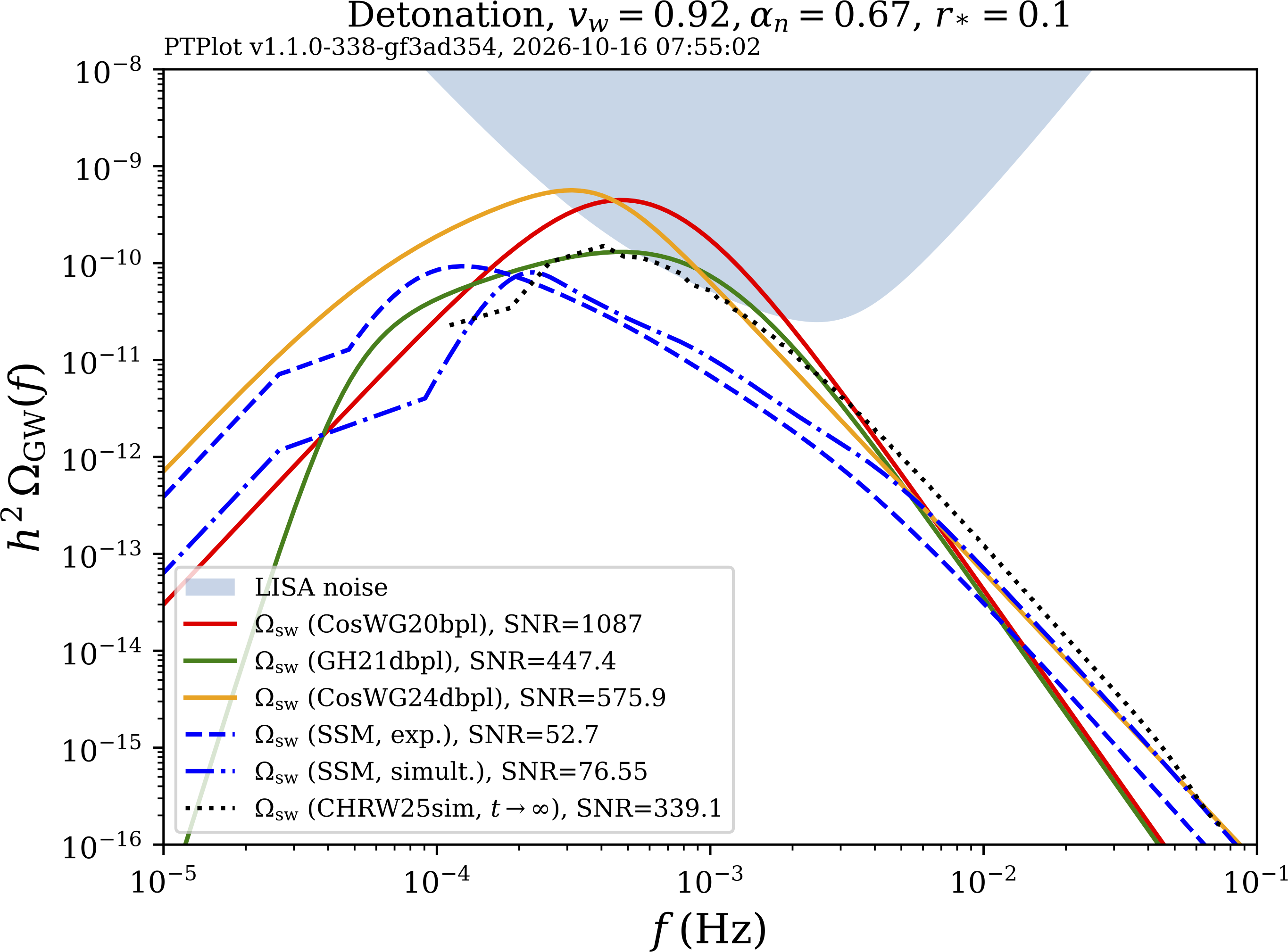
Courtesy Mika Mäki

Ansätze vs. simulation results 2

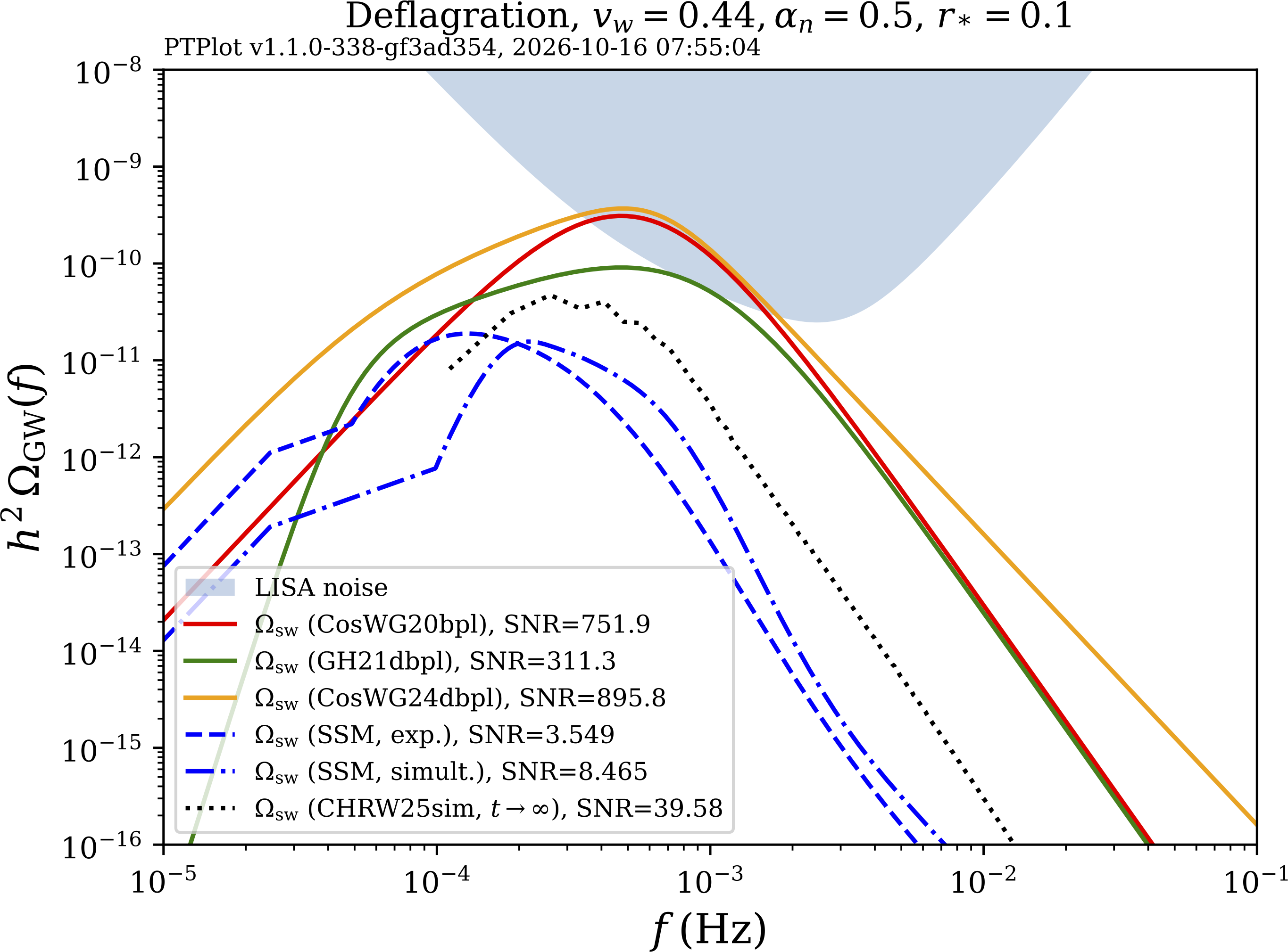
Courtesy Mika Mäki

Strong phase transition comparisons

Instantaneous GW production rate: arXiv:2505.17824

Detonation, $v_\mathrm{w} = 0.92$, $\alpha = 0.67$

Deflagration, $v_\mathrm{w} = 0.44$, $\alpha = 0.5$

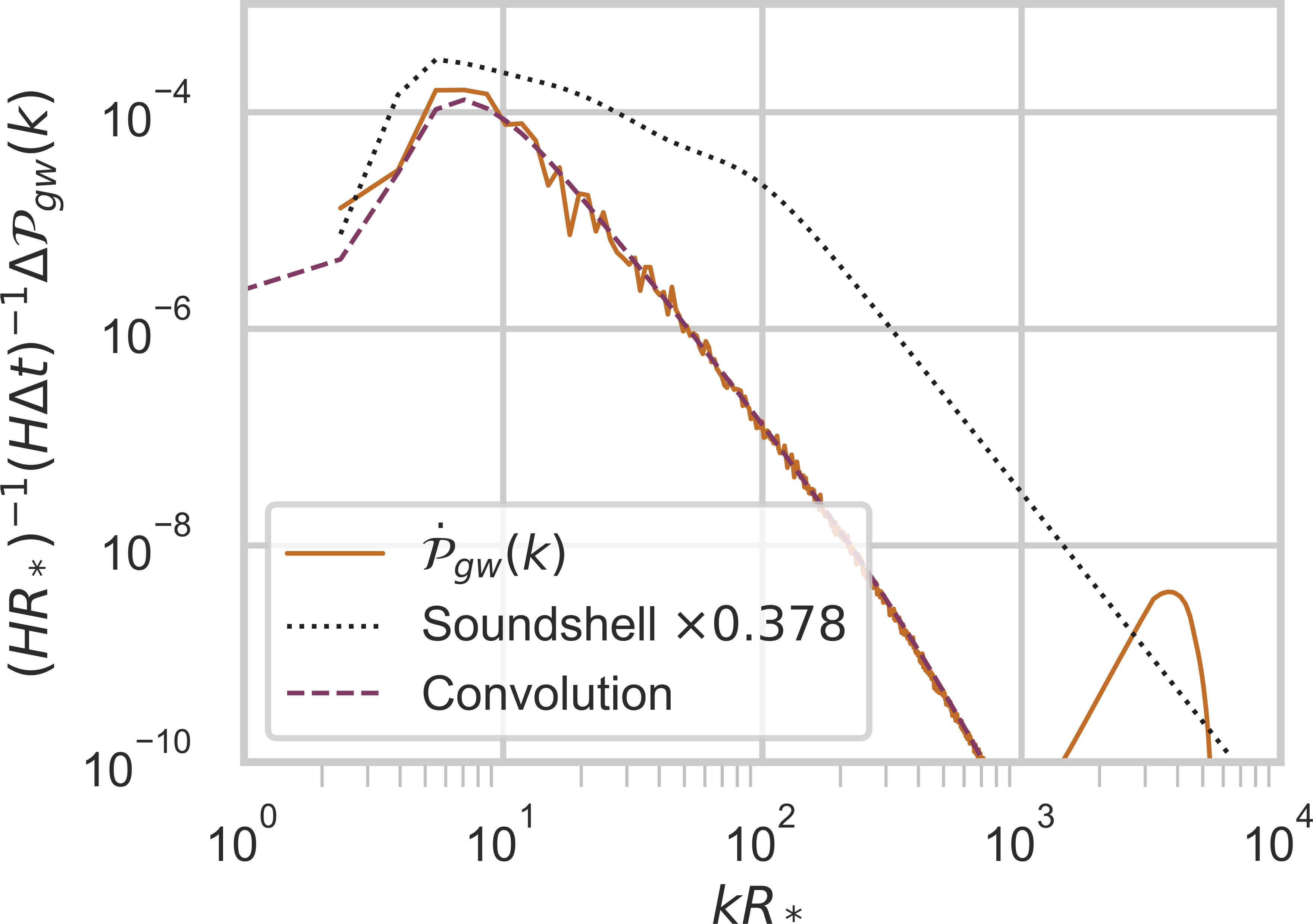
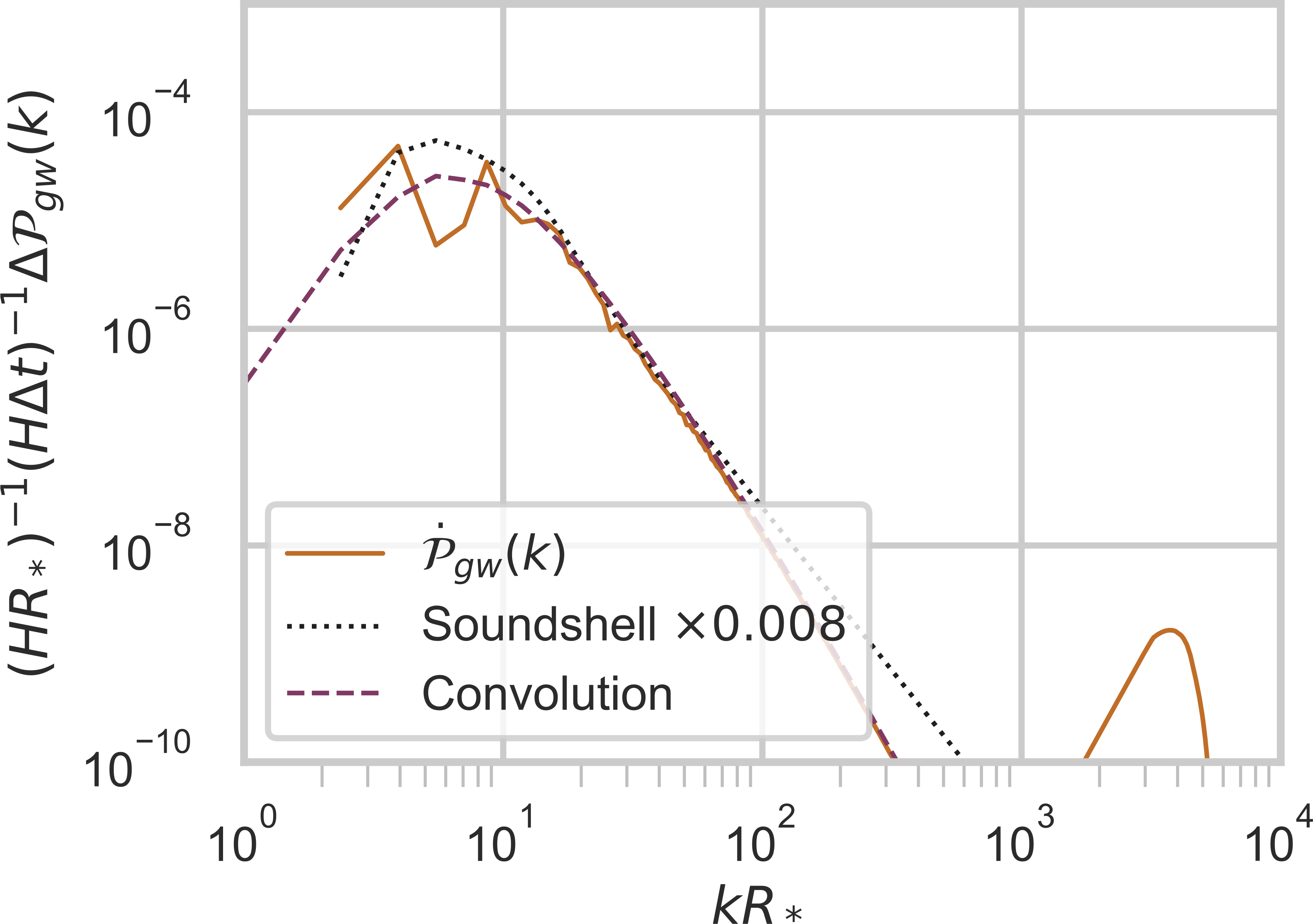
Sound shell model overestimates, gets wrong shape
Convolving fluid velocity power spectrum is better

Fluid velocity power $\mathcal{P}_U$

Separated into $\mathcal{P}_{U_\parallel}$ and $\mathcal{P}_{U_\perp}$ (enthalpy-weighted $u^\mu$)

Detonation, $v_\mathrm{w} = 0.92$, $\alpha = 0.67$

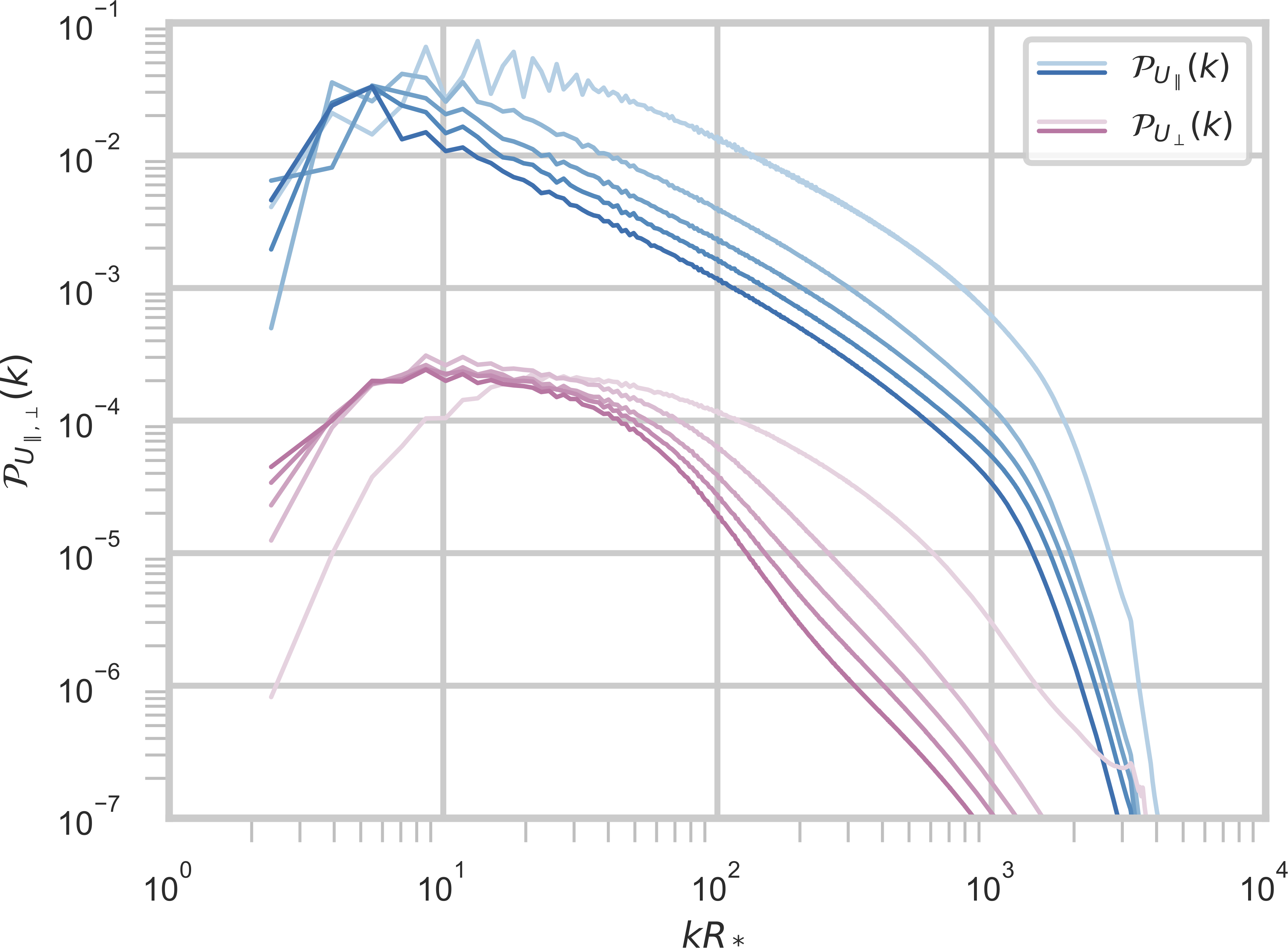Vortical $\ll$ compressional

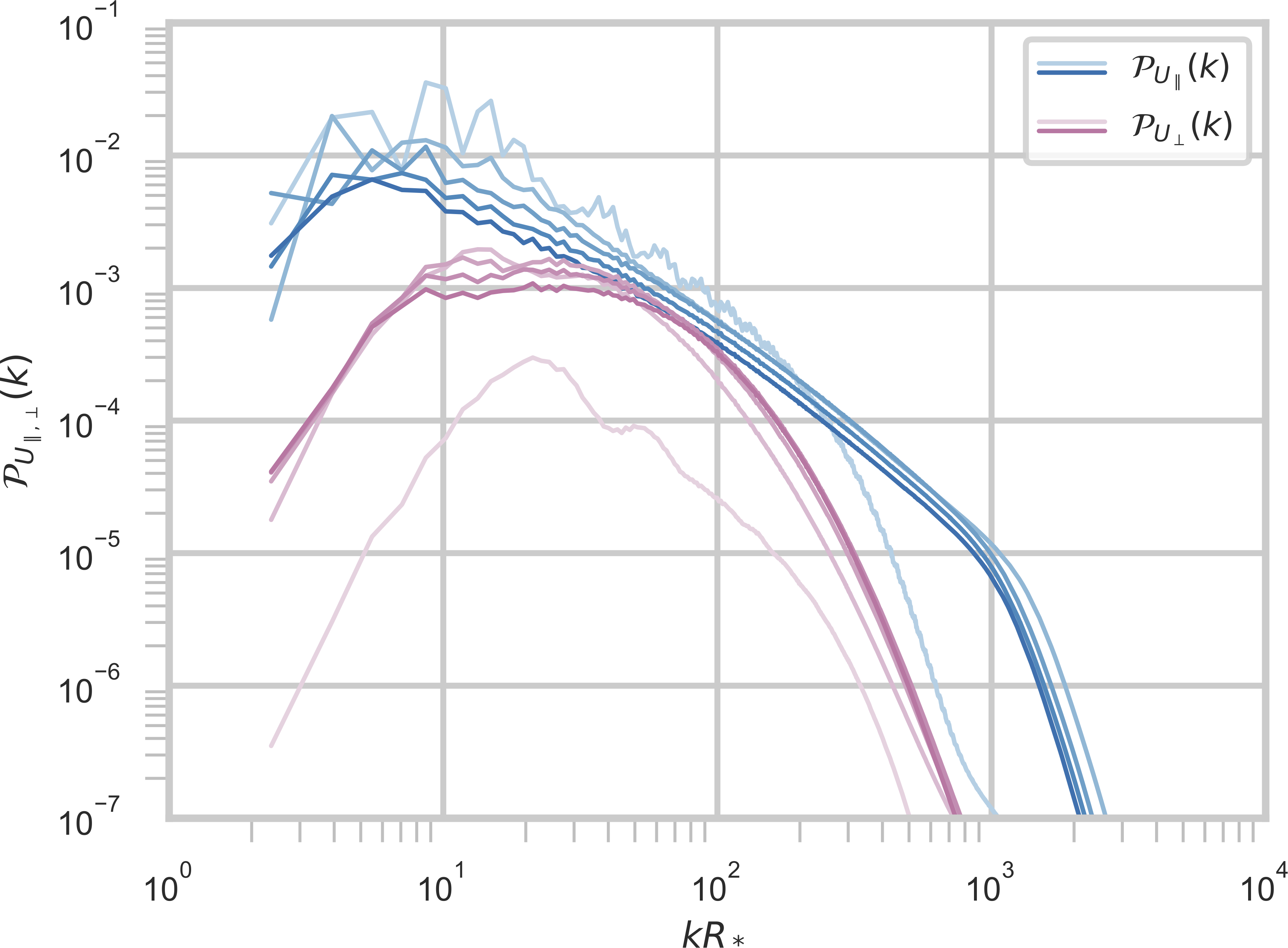Deflagration, $v_\mathrm{w} = 0.44$, $\alpha = 0.5$

Vortical $\sim$ compressional for some $k R_*$

Compressional modes

Shocks

⬇︎
⬇︎
⬇︎
KE decay

Kinetic energy decay

$U_\parallel = U_\parallel^\text{max}\left[1 + \Delta t/t_*\right]^{-\zeta/2}$; the prediction is $\zeta \approx 10/7$ from 2407.05826

Detonation, $v_\mathrm{w} = 0.92$, $\alpha = 0.67$

Deflagration, $v_\mathrm{w} = 0.44$, $\alpha = 0.5$

$\zeta = 1.48 \approx 10/7$

$\zeta = 0.86$

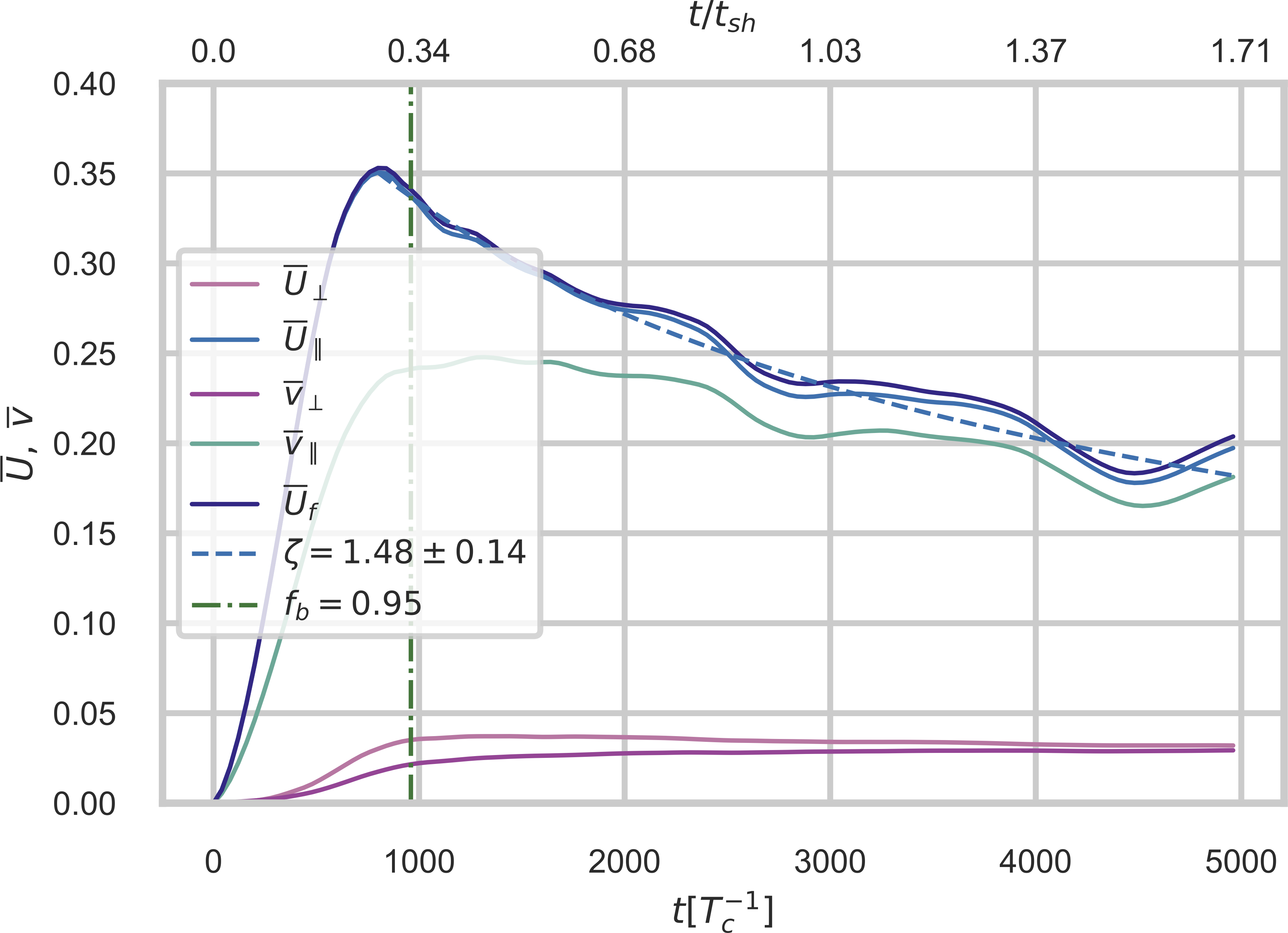
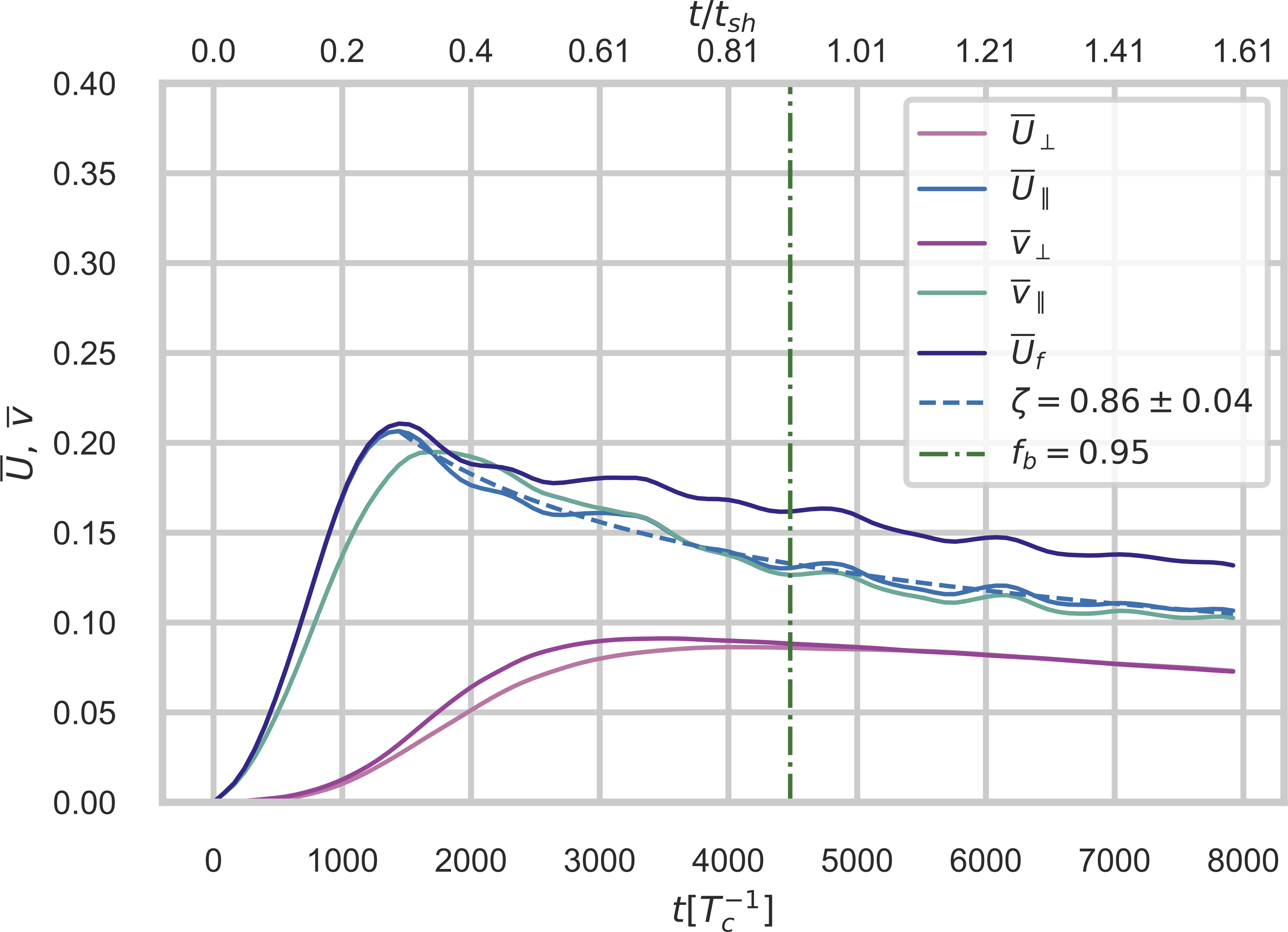
Higgsless: $\zeta \approx 10/7$ for deflagrations too 2409.03651
Could metastable phase heating be responsible?

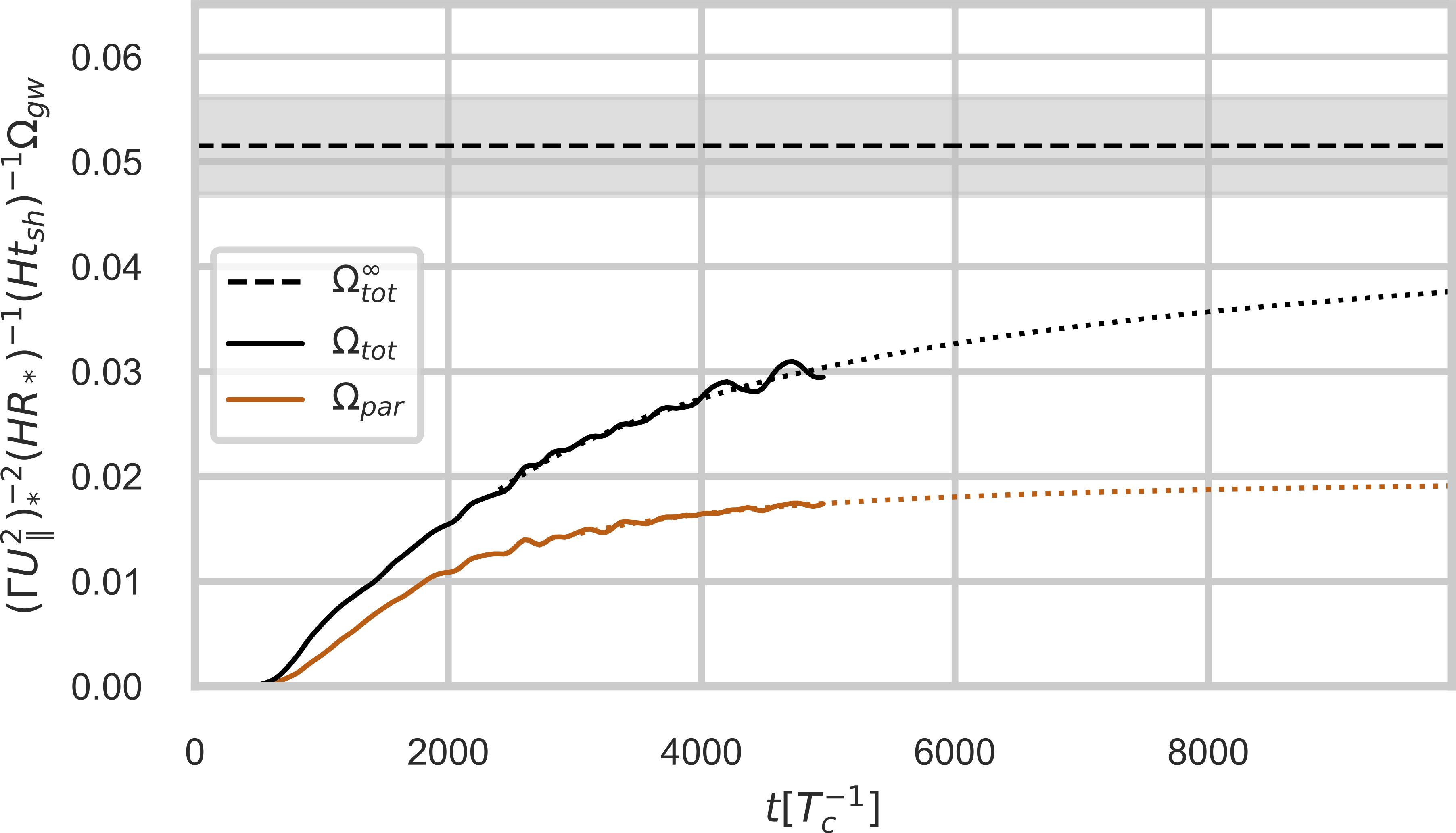
GW saturation

Asymptotic $\Omega_\text{gw}(t) = \Omega_\text{gw}^\infty \left[ 1- \left(\Delta t/t_*\right)^{-d}\right]$

Detonation
$v_\mathrm{w} = 0.92$, $\alpha = 0.67$

Deflagration
$v_\mathrm{w} = 0.44$, $\alpha = 0.5$

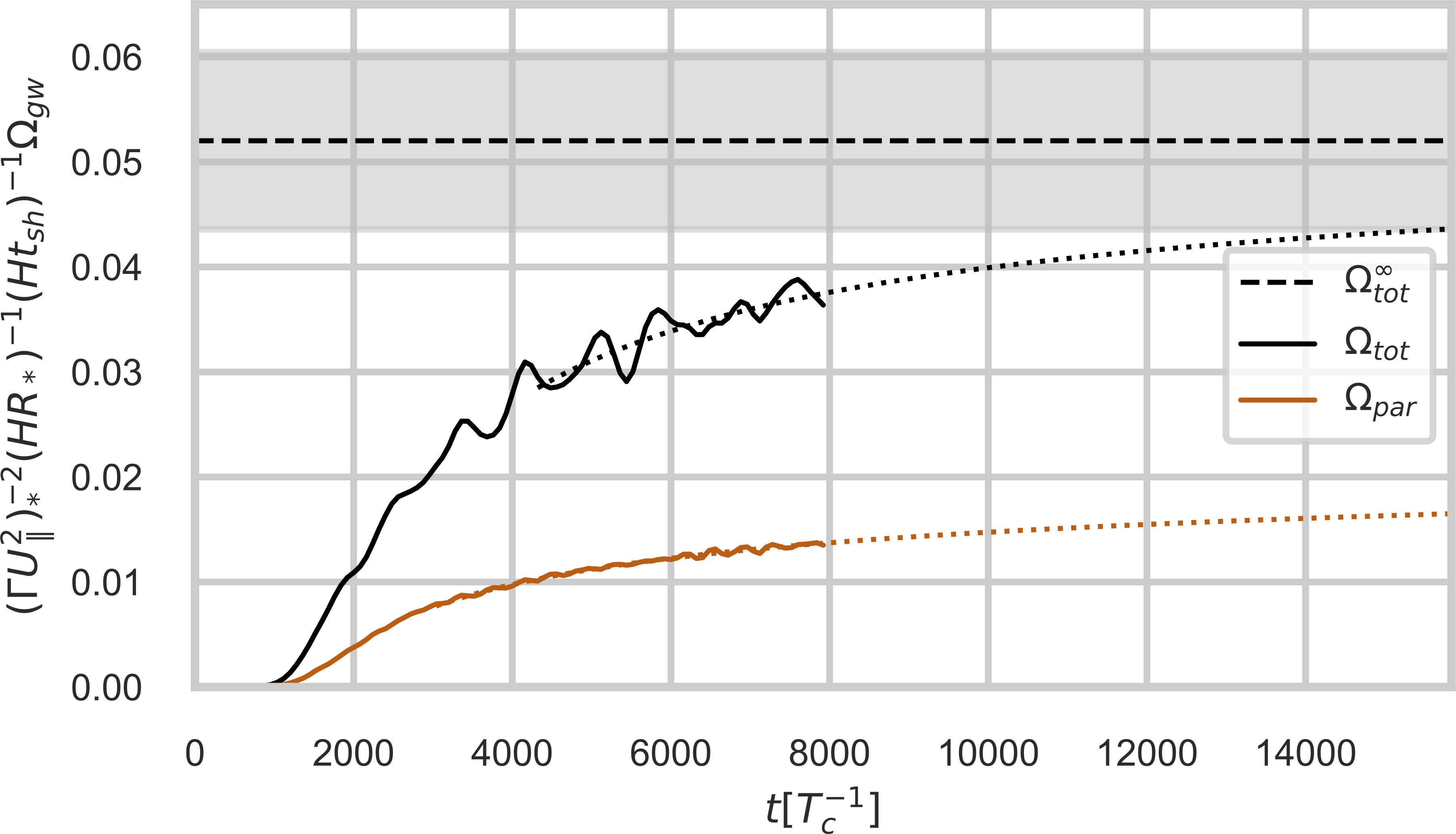
Can thus determine a dimensionless final 'efficiency' factor for GW production $\tilde{\Omega}_\text{gw}^\infty \approx 0.017$.

$d \approx 0.61$

$d \approx 0.79$

Compare velocity components

$P_\perp/P_\parallel$ for deflagration ($\alpha=0.5$, $v_\mathrm{w}=0.44$).

Field+fluid arXiv:2505.17824

Higgsless arXiv:2409.03651

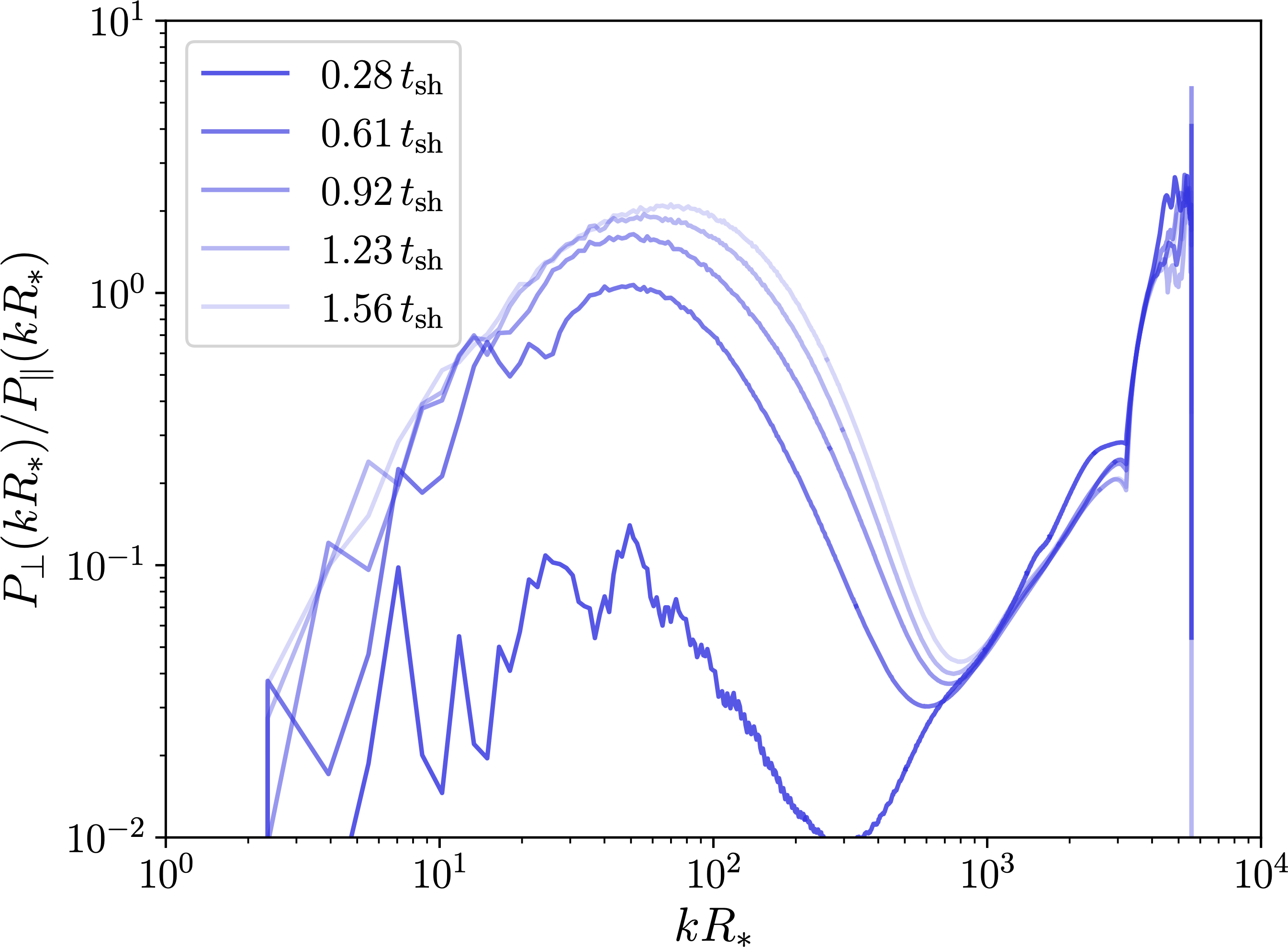
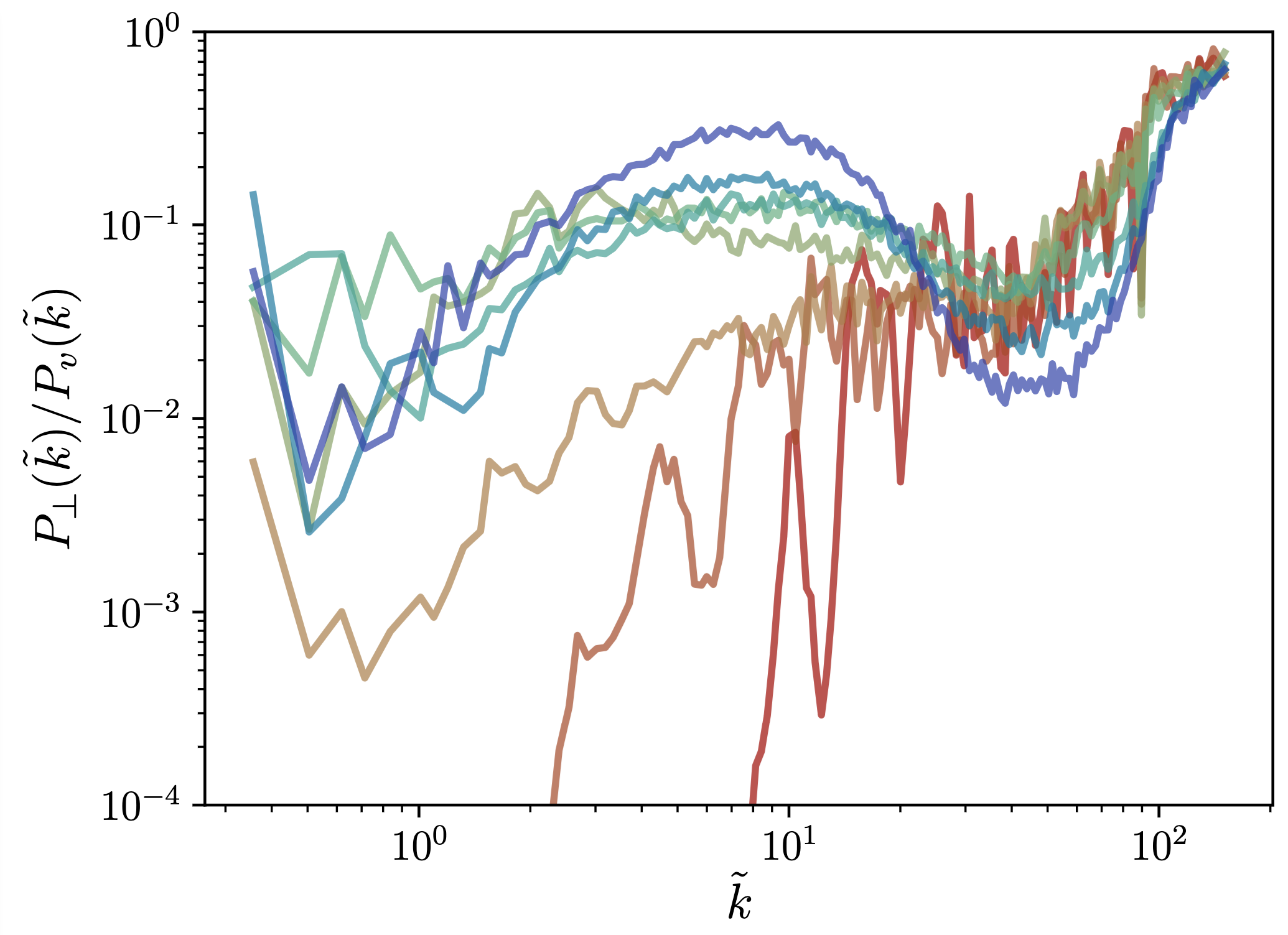
Higgsless sees a lot less rotational power
$\Rightarrow$ Vorticity generated during transition 1906.00480 etc.

Next: "deep field" ➢ "wide field"

Scan in $v_\mathrm{w}$, $\alpha$, $R_*$, ... – here is a sample:

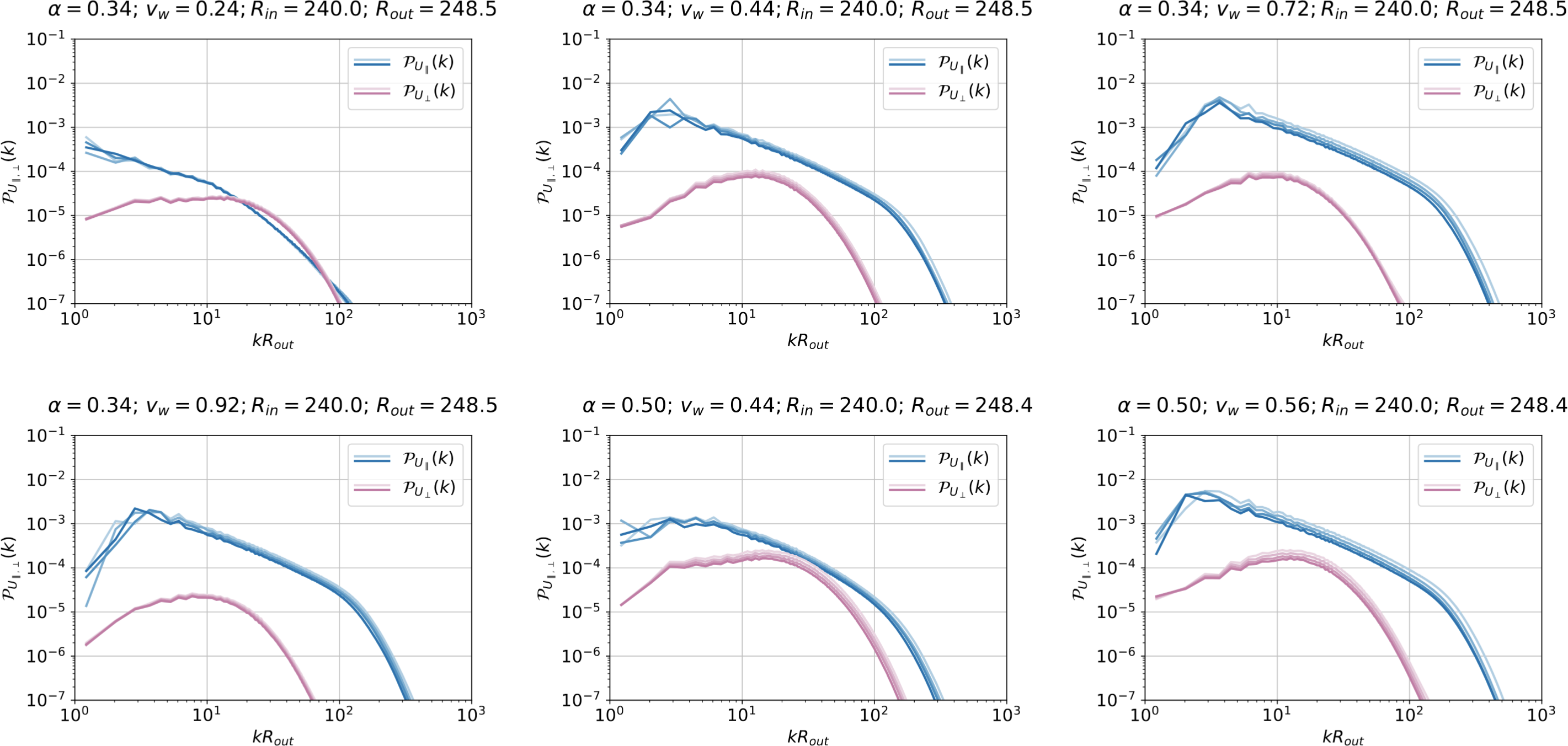
Including hybrids!

A plug

We are organising a COST action titled 'HIPPO'
(HIggs Pairs and POtential). Topics will include:

Complementarity between collider physics and gravitational wave cosmology
Improving the accuracy of predictions of stochastic cosmological backgrounds from BSM physics
Providing public tools to analyse data
Sharing expertise collider physics ⇋ GWs/cosmology (e.g. machine learning)

Conclusions

We have extended our earlier simulation-based studies to strong phase transitions
Even with various phenomenological corrections, ansätze do not work well for strong transitions
See evidence for turbulent motion in both compressional and longitudinal modes
For strong phase transitions with short duration compared to Hubble damping, can extrapolate $\Omega_\text{gw}^\infty$

And a question to get you started:

Is there any evidence of non-Gaussianity?