
Primordial sources of gravitational waves:
what can simulations teach us?
David J. Weir [they/he]
-
University of Helsinki
davidjamesweir@mementomori.social
This talk: saoghal.net/slides/heidelberg2026
Physics Graduate Days, 7-10 April 2026
Day 1
Introduction
Housekeeping
- Participant list
- Lecture note writing team
Today
- Introduction to the course
- First order phase transitions
- Lattice Monte Carlo for phase transitions
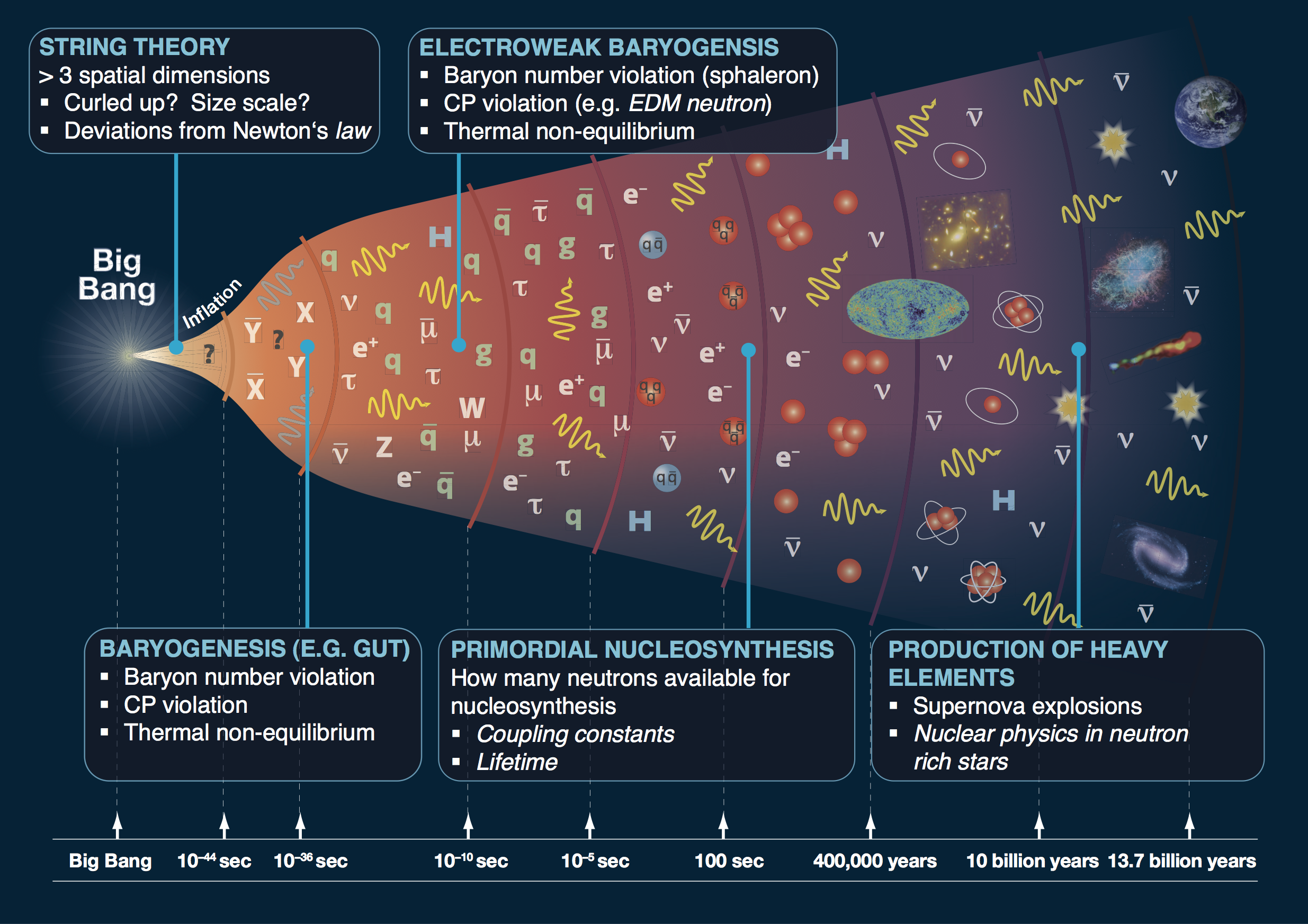
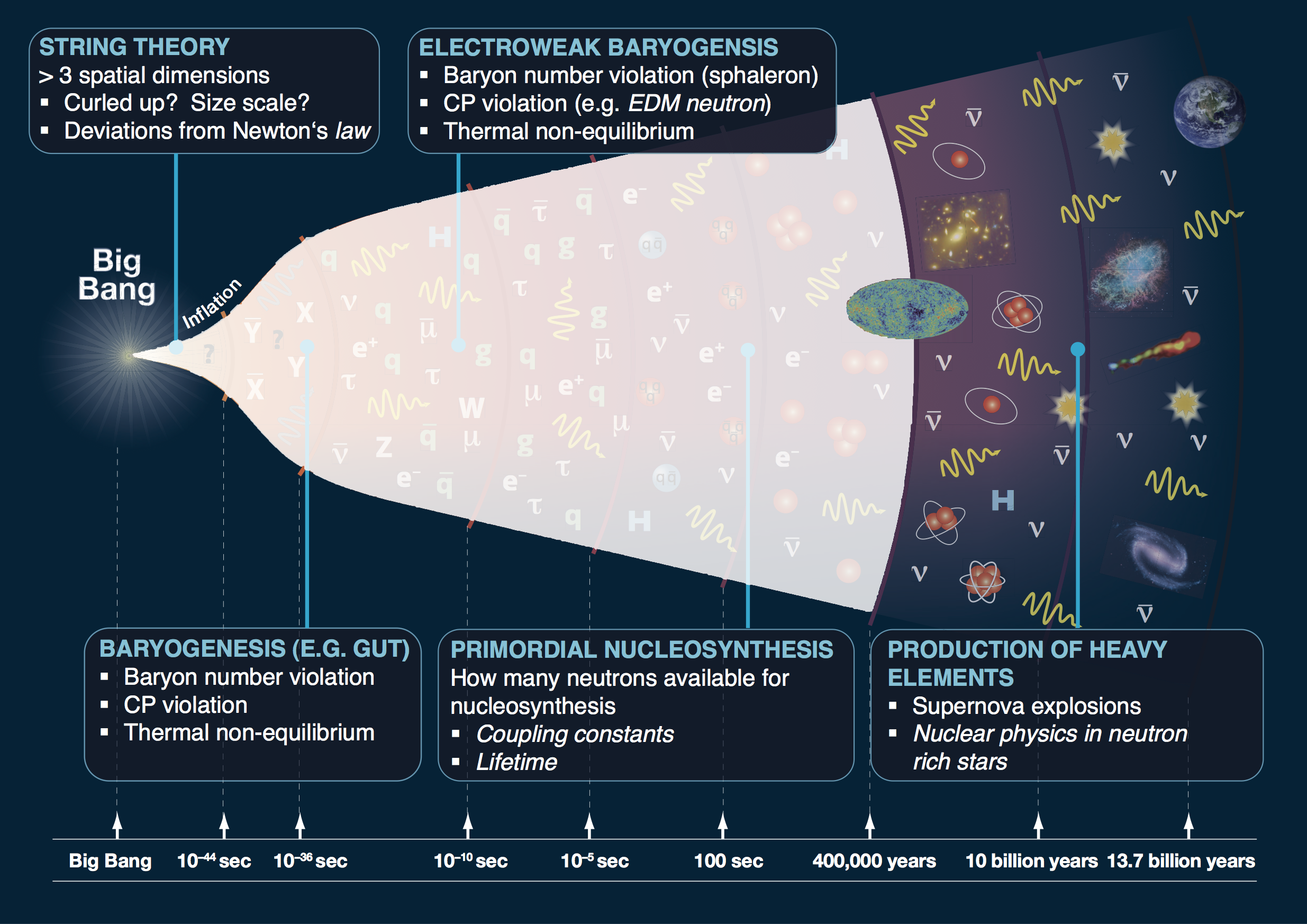
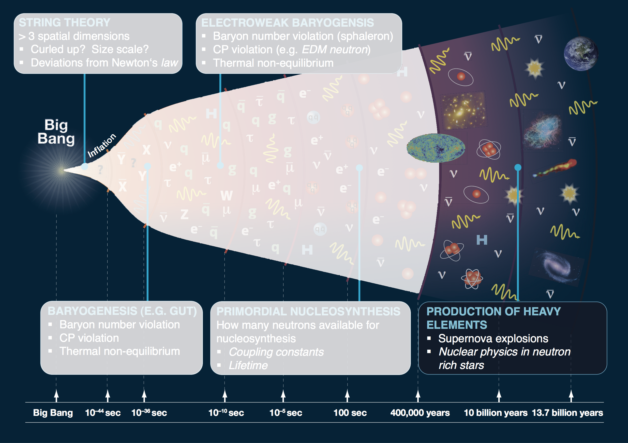
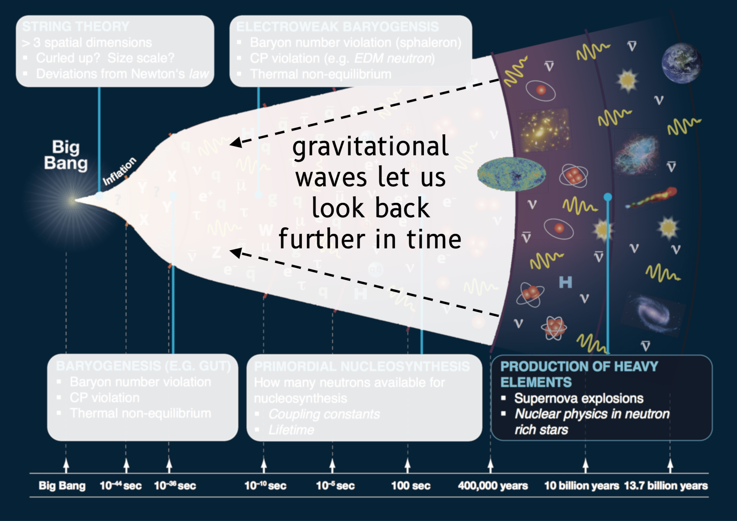
What happened in the early universe? before recombination? in dark sectors?
About me
- Since 2024: Professor of GW cosmology in Helsinki
- My focus: simulating early universe phase transitions
- Simulating theories beyond the Standard Model
- Lattice Monte Carlo simulations (not really QCD)
➡︎ investigate phase diagrams, parameters
- Lattice Monte Carlo simulations (not really QCD)
- Simulating the phase transition process itself
- 'Real time' simulations (relativistic hydro, etc.)
➡︎ compute GW power spectrum, etc.
- 'Real time' simulations (relativistic hydro, etc.)
- Also: simulating gravitational wave detectors (LISA)
- Want to see if a primordial signal could be seen
- Simulating theories beyond the Standard Model
We'll look at all of these things in this week's lectures
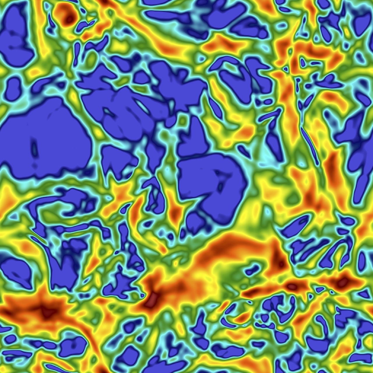
Monte Carlo simulation example
A nucleating bubble
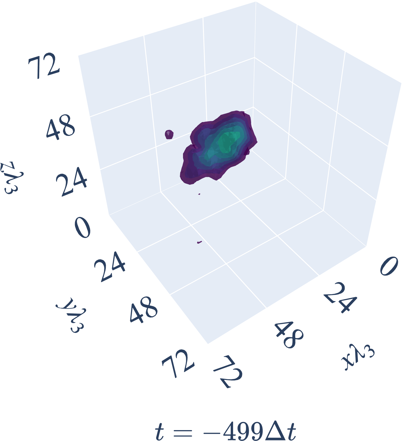
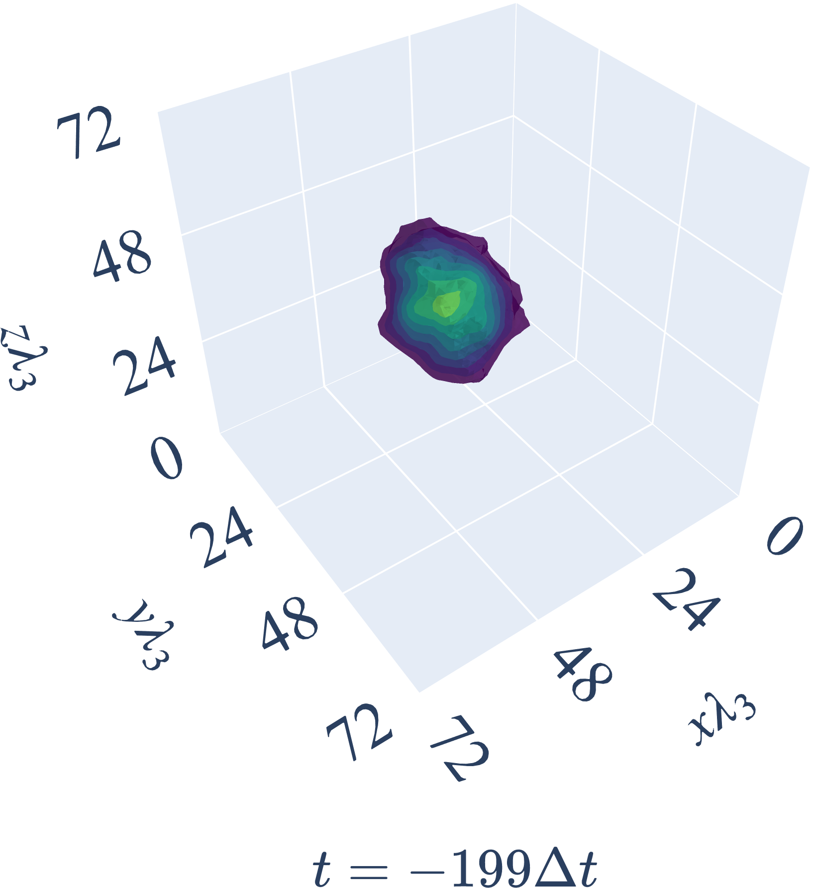
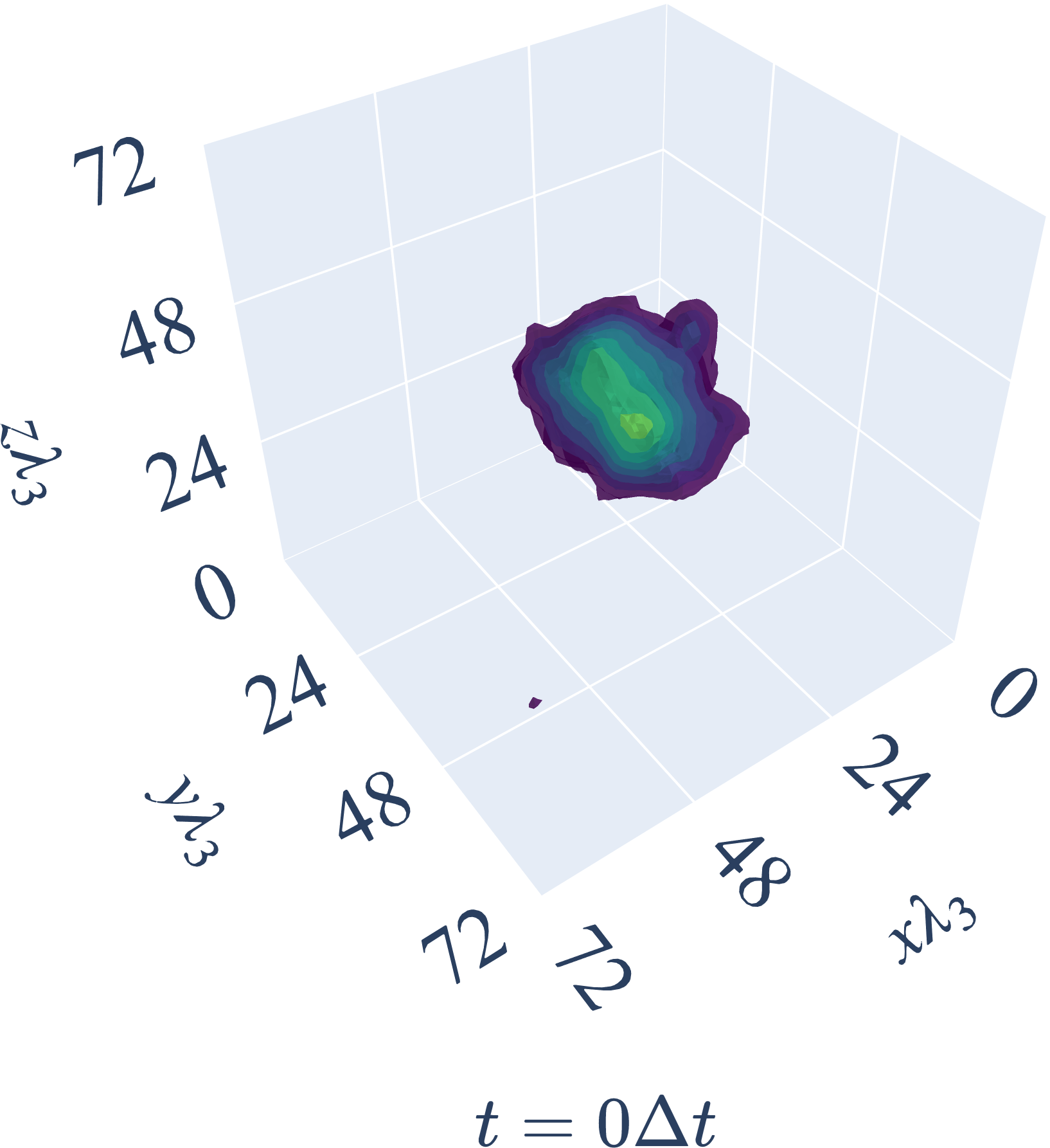
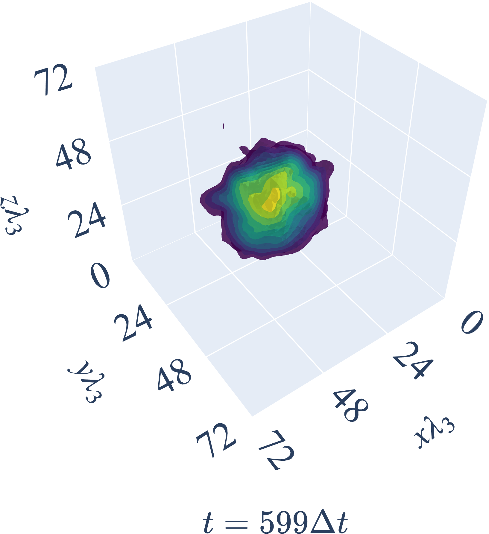
Created by Anna Kormu, arXiv:2404.01876
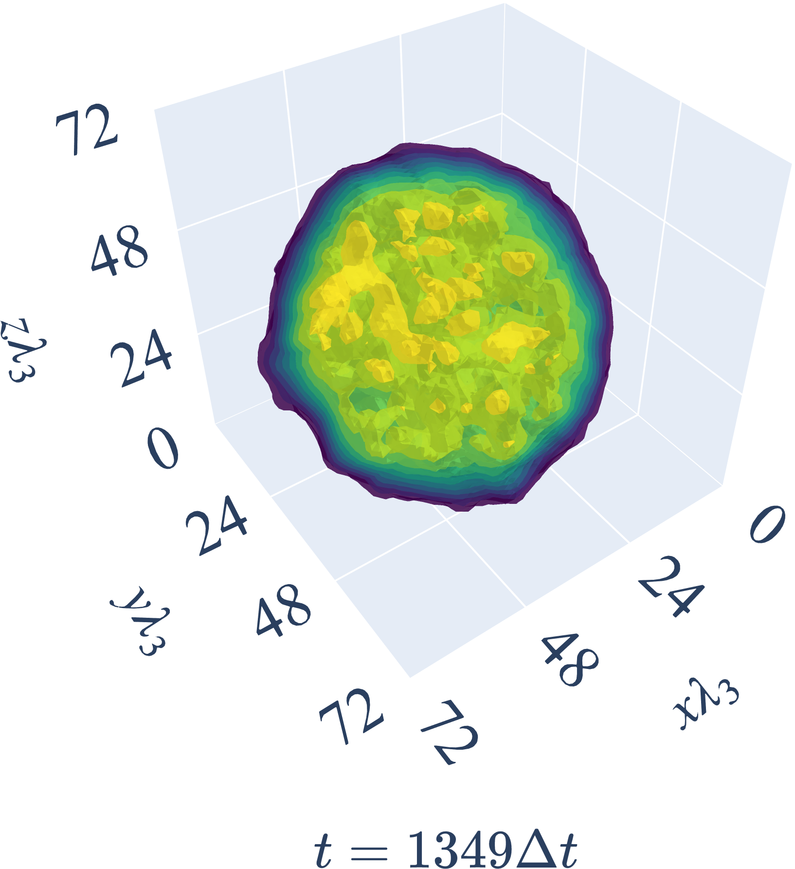
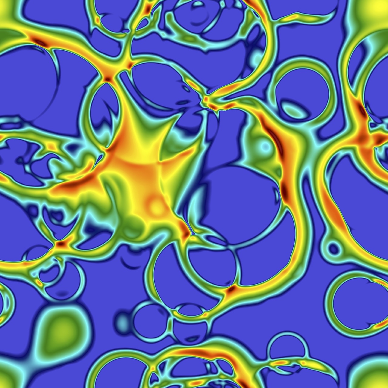
Real time simulation example
A strong phase transition
GW detector simulation example
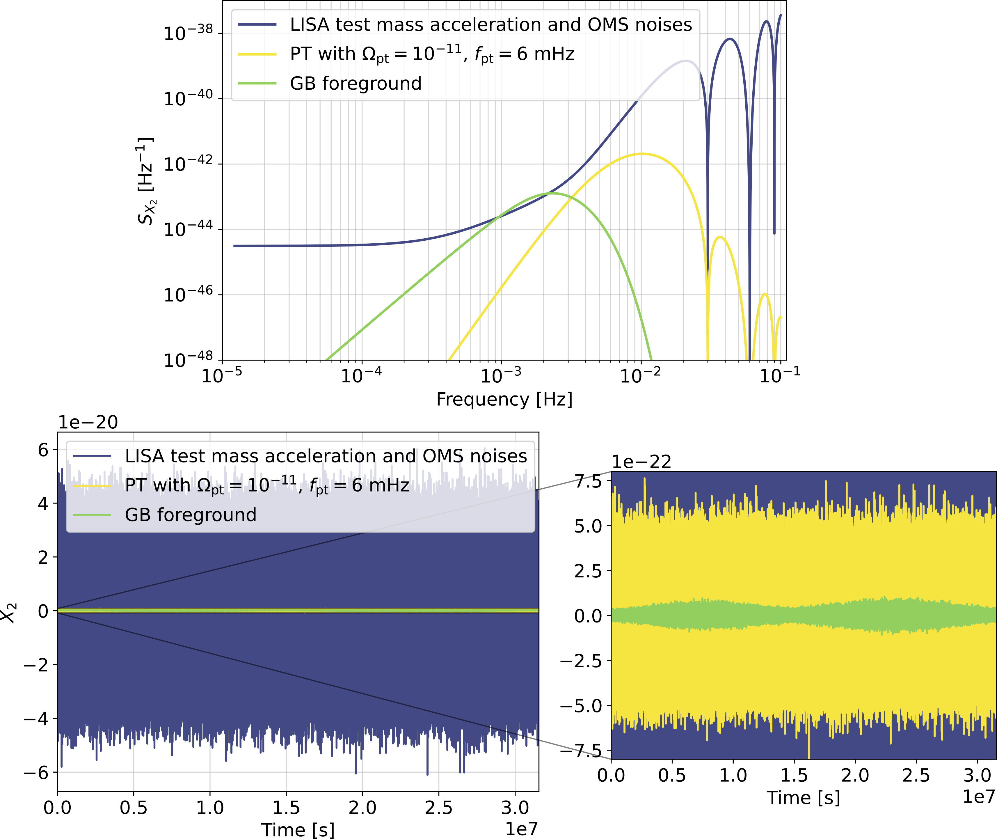
Created by Tiina Minkkinen, arXiv:2406.04894
About you ...

Learning outcomes for the course
After participating in this course, you should be able to:
- Justify the phenomenological interest in early universe phase transitions
- Describe simulation methods used to study phase transitions
- [Obtain a stress-energy tensor for GWs]
- Redshift a primordial stochastic GW source to today
- Explain how phase transitions source GWs
- Describe how GWs can be (directly) detected and how (for example) LISA will work
Methods
- Mixture of slides, and writing on tablet, and practical work with Jupyter notebooks:
- Notebooks at:
github.com/davidjamesweir/2026-lecture-demos - Jupyter notebooks work best on your own laptop, but they are tested to be usable on mybinder.org
- To keep things moving, we skip over most details
- Please go through derivations yourself
- Interaction tools like Presemo (and possibly Padlet)
- Please contribute (and have fun!)
What is a first-order phase transition?
(First-order) phase transitions
- During a phase transition certain thermodynamic properties change
- In a first-order phase transition...
- We see discontinuities in e.g. the energy density, pressure; there should be an order parameter
- Latent heat is released
- The transition completes by bubbles nucleating and expanding to fill the system
Assumptions for now:
- The phase transition arises from a cooling system (e.g. the early universe).
- The field undergoing the transition can be modelled by a scalar field $\phi$.
- Thermal, rather than quantum, fluctuations are dominant.
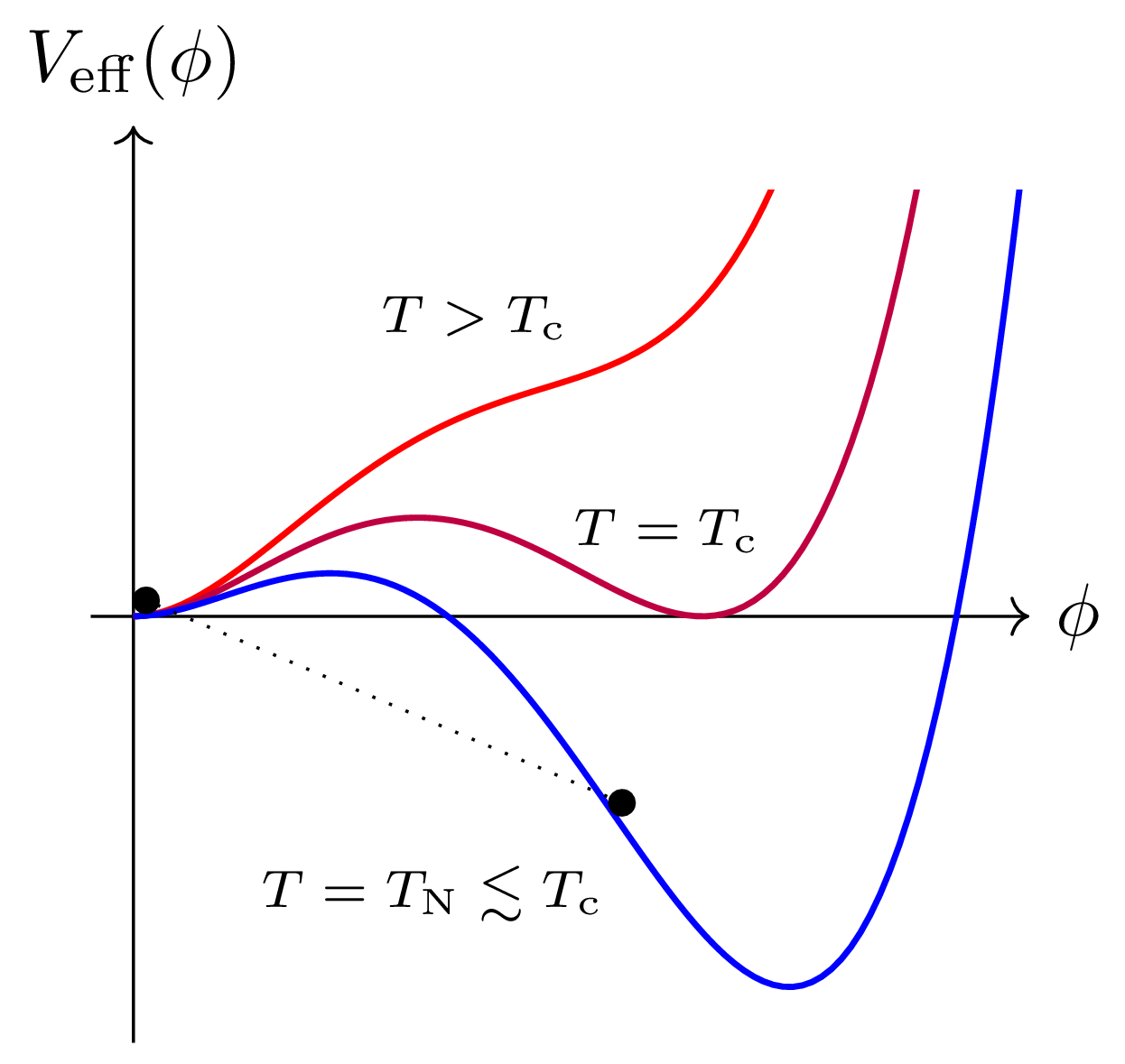
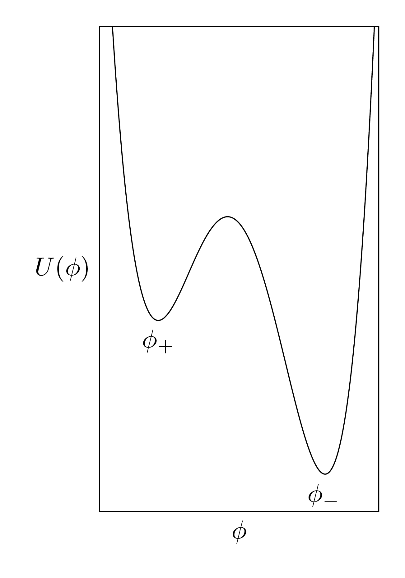
Field theory - effective potential
- High temperatures: potential has one global minimum
- At critical temperature $T_\mathrm{c}$: two minima and a barrier
- Below $T_\mathrm{c}$, second minimum becomes global minimum
- Nucleation temperature $T_\mathrm{N}$: bubbles 'start' to tunnel
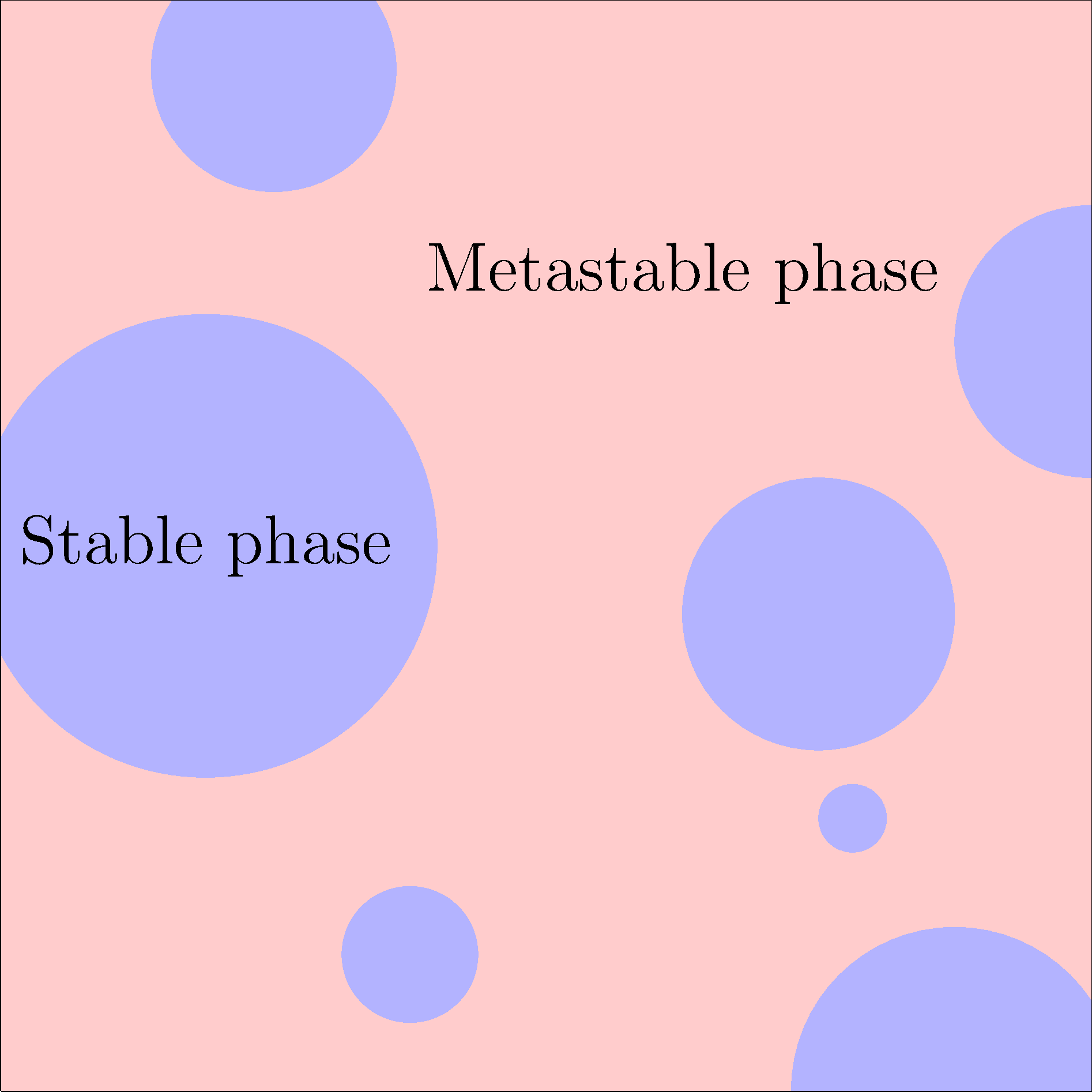
"Order parameter"
Distinguishes between the two phases - ideally zero in one and nonzero in the other, e.g. $\langle\phi\rangle$ or $\langle \phi^2 \rangle$ here.
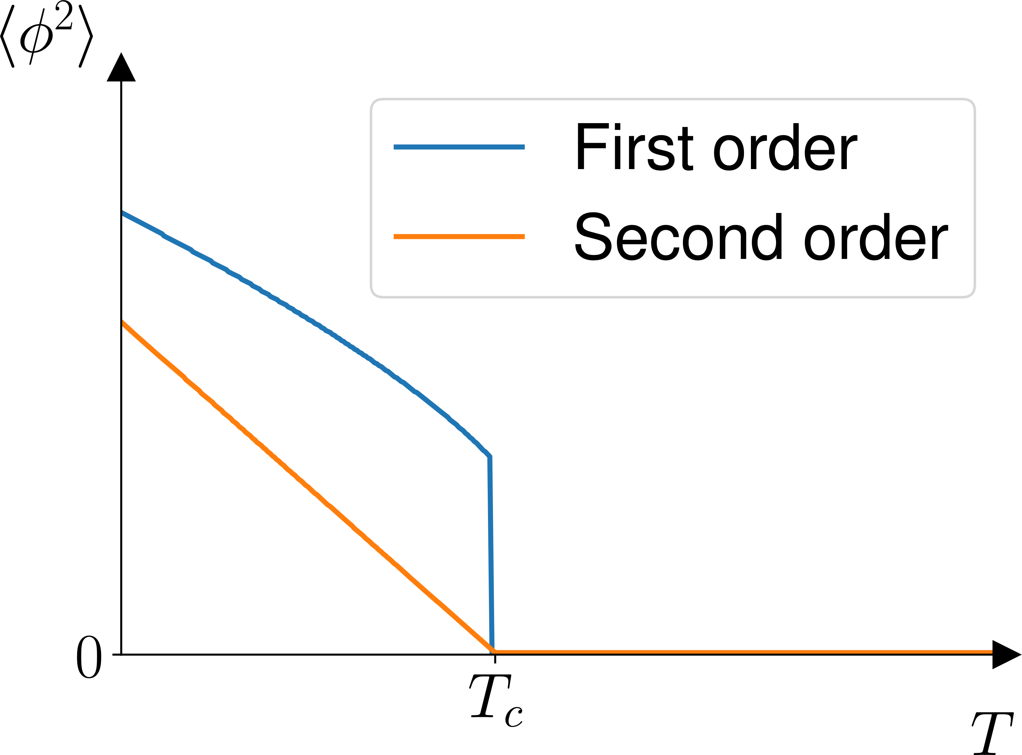
(crossover is even smoother, $C^\infty$ at $T_c$)
We'll often label a generic (pseudo-)order parameter $\theta$.
Once the bubbles have nucleated...
- Energy ('latent heat') is released during the transition
- This forces the bubble walls to expand
- Bubble walls accelerate (and, if there are suitable couplings, the cosmic fluid is heated through friction)
- Colliding bubbles, and perturbations in the cosmic fluid, source gravitational waves
Summary: what happens?
- Bubbles nucleate (temperature $T_\mathrm{N}$, on timescale $\beta^{-1}$)
- Bubble walls expand in a plasma (at velocity $v_\mathrm{w}$)
- Reaction fronts form around walls (with strength $\alpha$)
- Bubbles + fronts collide GWs
- Sound waves left behind in plasma GWs
- Shocks [$\rightarrow$ turbulence] $\rightarrow$ damping GWs
Impact of PT parameters
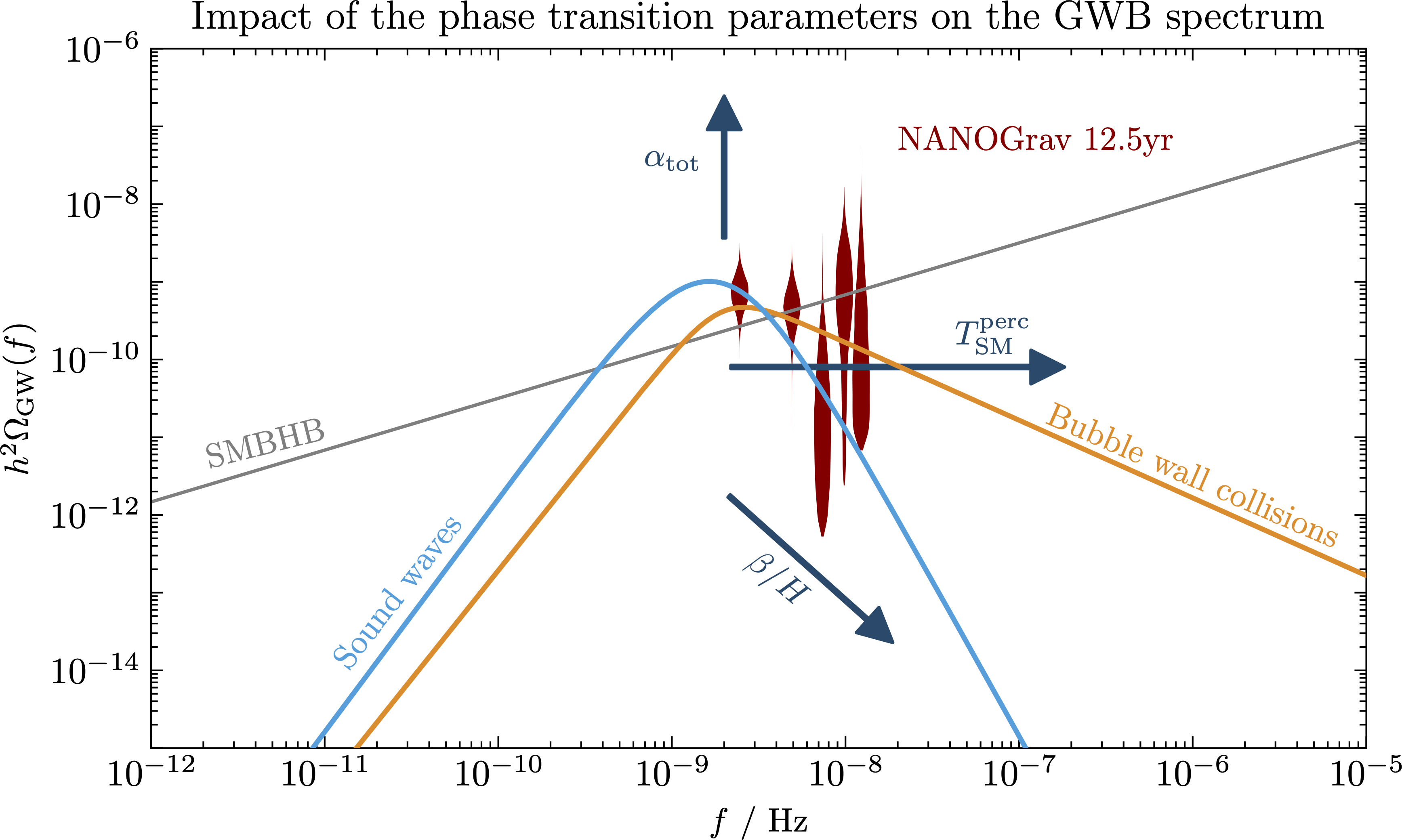
From arXiv:2306.09411
Why are early universe phase transitions interesting?
- Bubbles colliding generate potentially observable signatures, e.g. a stochastic background of gravitational waves
- A period of out-of-equilibrium physics can facilitate e.g. dark matter production, or creation of a baryon asymmetry.
Gravitational waves and new physics
First-order phase transitions are therefore a
- Out of sight of particle physics experiments (e.g. dark matter candidates and dark sectors), or
- At higher energy scales than colliders can reach.
There are many models based on the above concepts.
Let us instead look at the 'traditional' motivation for a primordial phase transition, electroweak baryogenesis.
Baryon asymmetry of the universe
- Everyday experience: more baryons than antibaryons
- Quantify this through the asymmetry parameter $$ \eta = \frac{n_B - n_\overline{B}}{n_\gamma}$$
- From Planck, we have $\eta = (6.10 \pm 0.04) \times 10^{-10}$ excess baryons per photon
- This sounds small... but it's not!
Deriving $\eta$
- We need the Friedmann equation... $$\rho_c = \frac{3 H_0^2}{8 \pi G}$$
- ... the photon number density today $n_\gamma = 2 \zeta(3) T_0^3 / \pi^2$
- ... mean mass per baryon $\langle m \rangle \approx
m_\mathrm{p}$
( but smaller due to Helium binding) - ... and $\Omega_\mathrm{B} h^2 = 0.02207 \pm 0.00033 = h^2 \rho_\mathrm{b}/\rho_c$
- Then the asymmetry parameter $$\eta = \frac{\rho_c \Omega_\mathrm{B}}{\langle m \rangle n_\gamma}.$$
Sakharov conditions
- Assume $B=0$ in (very) early universe; $B>0$ later.
- In 1967 Andrei Sakharov (implicitly) wrote down the
necessary conditions for baryogenesis:
- Baryon number $B$ violation
- $C$ and $CP$ violation
- Departure from thermal equilibrium
- These specify only what is needed, not how it works.
About the Sakharov conditions: $C$
- Note that if we had $B$ violation without $C$ violation, then $\overline{B}$ violation would occur at the same rate: $$ \Gamma(X \to Y + B) = \Gamma(\overline{X} \to \overline{Y} + \overline{B}) $$
- Thus over time $B=0$ still, unless we have $C$ violation too: $$ \frac{\mathrm{d} B}{\mathrm{d} t} \propto \Gamma(\overline{X} \to \overline{Y} + \overline{B}) - \Gamma(X \to Y + B).$$
About the Sakharov conditions: $CP$
- In fact, also need $CP$ violation
- Consider $B$-violating $X \to q_\mathrm{L} q_\mathrm{L}$ process making left handed baryons
- $CP$ symmetry turns this equation into $ \bar{X} \to \bar{q}_\mathrm{R} \bar{q}_\mathrm{R}$
Electroweak baryogenesis
Kuzmin, Rubakov, Shaposhnikov
- Assume that there was no net baryon charge before the $\mathrm{SU}(2)_L \times \mathrm{U}(1)_Y \to \mathrm{U}(1)_\text{EM}$ breaking
- Processes that take place as the Higgs boson becomes massive responsible for creating a net baryon number
- Basically needs a first order phase transition to be successful (exceptions exist)
- Baryons produced through the anomaly $$ \begin{multline} B(t) - B(0) = 3[N_\text{cs}(t) - N_\text{cs}(0)] \\ = 3\int \mathrm{d} t \int \mathrm{d}^3x \frac{1}{16\pi^2} \mathrm{Tr} \, F_{\mu\nu} \tilde{F}^{\mu\nu}. \end{multline}$$
Illustration
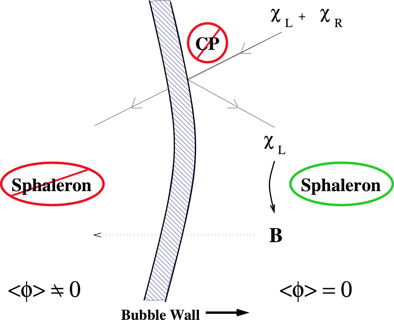
EW BG and the Sakharov conditions
Baryogenesis satisfies the Sakharov conditions:- $C$ and $CP$ violation: occurs due to particles scattering off bubble walls.
- $B$ violation: the $C$ and $CP$ violation means that sphaleron transitions in front of the wall produce more baryons than antibaryons.
- Out of equilibrium: the bubble walls (and sound shells) disturb the symmetric-phase equilibrium state.
The bad news (sort of)
- There is no evidence for a phase transition in the (minimal) Standard Model
- Electroweak + QCD phase transitions are crossovers
- Thus:
- Electroweak baryogenesis does not work without modifications or extra fields
- No significant source of a stochastic background of gravitational waves in the Standard Model
- Interest is therefore focussed on extensions of the Standard Model where there are phase transitions
- ... but how do we know the electroweak phase transition is a crossover?
EW PT in the SM
Work in the 1990s found this phase diagram for the SM:
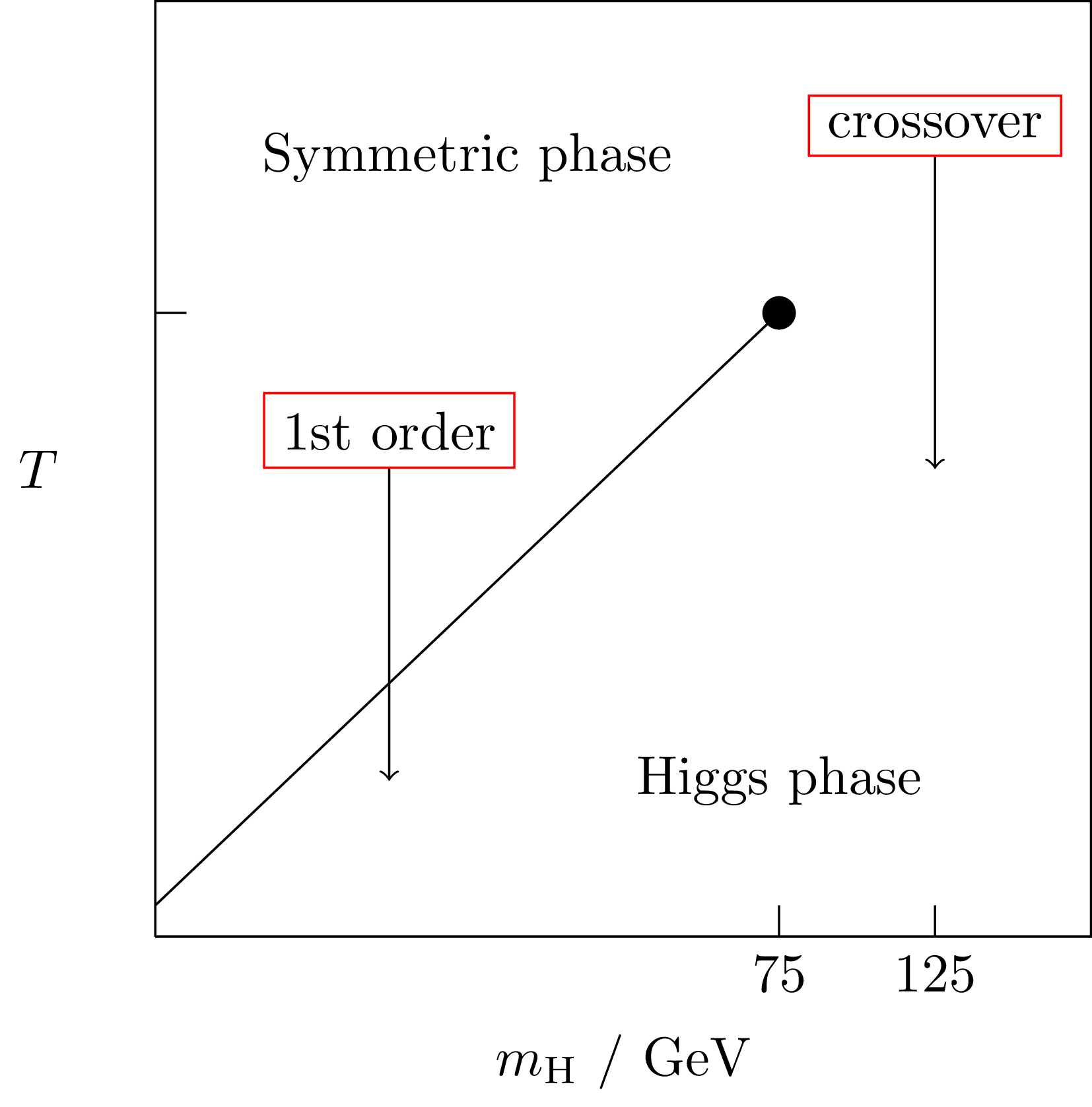
At $m_H = 125 \, \mathrm{GeV}$, SM is a crossover
Kajantie et
al.; Gurtler et al.;
Csikor et al.;
...
Using dimensional reduction
- At high $T$, system looks 3D at distances $\Delta x
\gg 1/T$

- Match Green's functions at each step to desired order
- Heavy fields are integrated out, leaving light fields to be studied on the lattice arXiv:hep-ph/9508379
- This avoids 'infrared problems' inherent in thermal field theory.
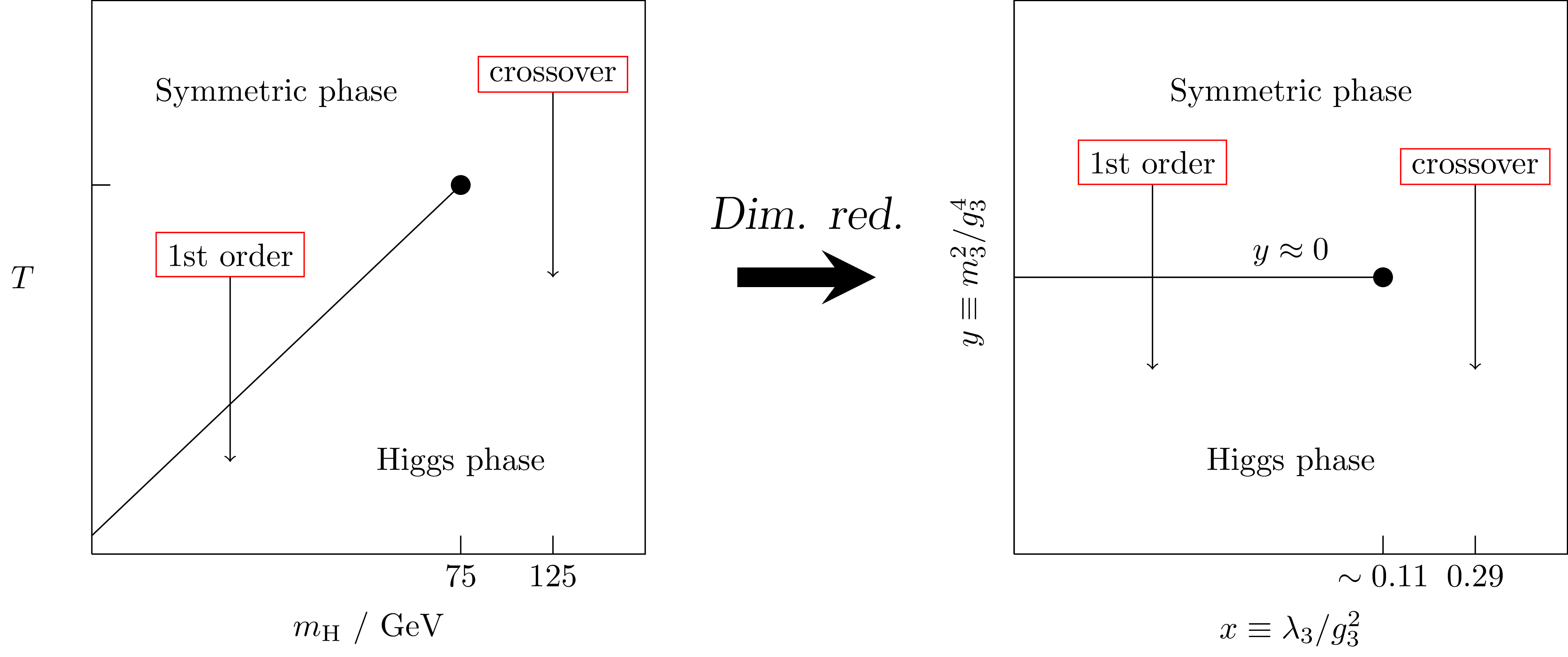
Dimensional reduction
- Decomposition of fields (Matsubara modes): $$ \phi(x,\tau) = \sum_{n=-\infty}^{\infty} \phi_n(x) e^{i \omega_n \tau}; \qquad \omega_n = 2n\pi T $$
- Integrate out $n\neq 0$ modes due to the scale separation $$ \begin{align} Z & = \int \mathcal{D} \phi_0 \mathcal{D} \phi_n e^{-S(\phi_0) - S(\phi_0, \phi_n)} \\ & = \int \mathcal{D} \phi_0 e^{-S(\phi_0) - S_\text{eff}(\phi_0)} \end{align}$$
- The 3D theory (with most fields integrated out) is easier to study, has fewer parameters!
Using the dimensional reduction
- Study the DR'ed 3D theory with lattice simulations.
- Done in the 1990s for the
Standard Model:
![]()
- [Q: Can we map other theories to same 3D model?]
SM is a Crossover
At $m_H = 125 \, \mathrm{GeV}$, $T_\mathrm{c} = 159.5 \pm 1.5 \, \mathrm{GeV}$
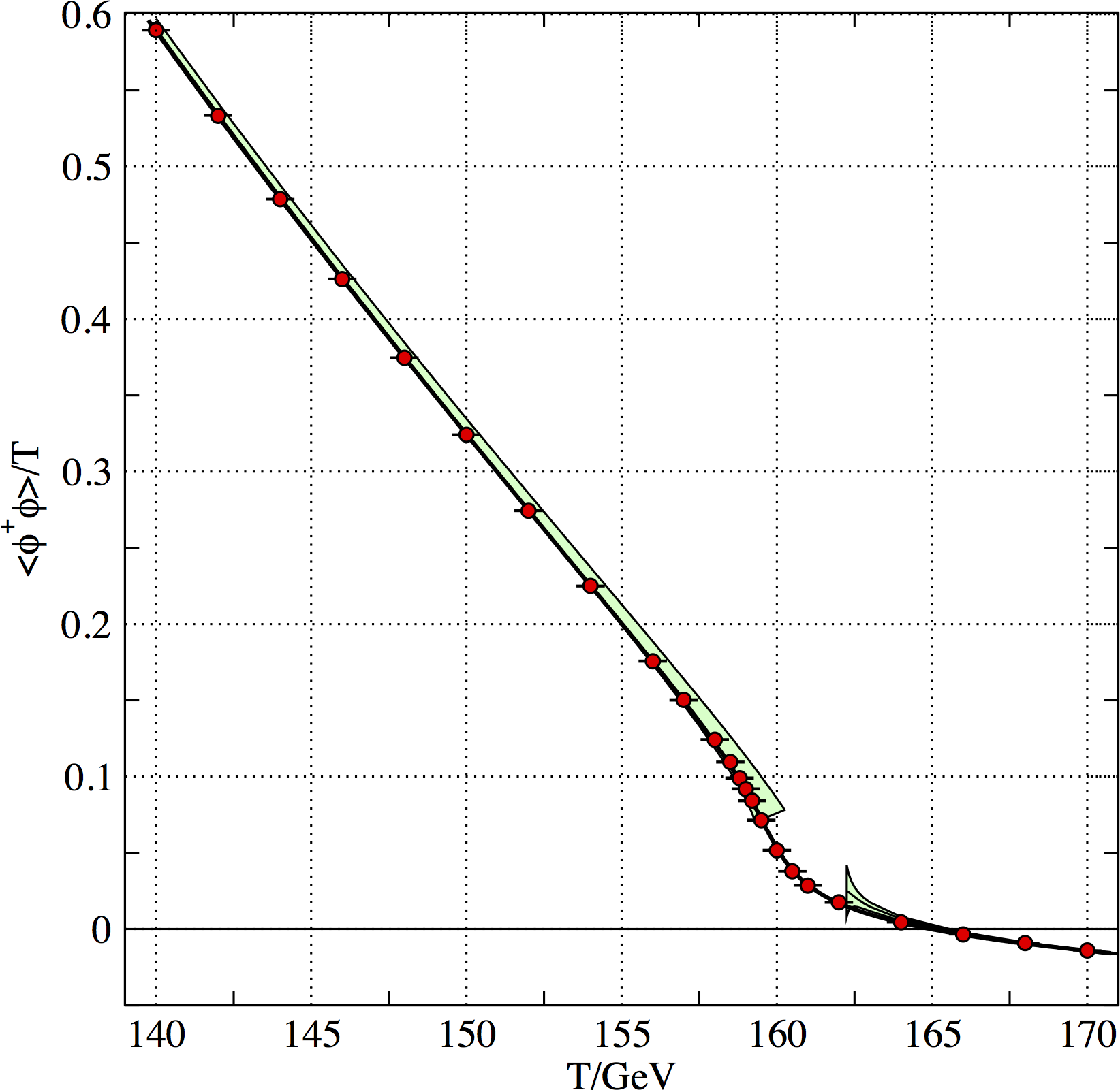
Source: D'Onofrio and Rummukainen
Applying lattice methods to extensions of the Standard Model
- Can add extra fields (a singlet $\phi$, a triplet $\Sigma$, etc.) to Standard Model.
- Choose suitable parameters, can get a first-order phase transition again.
- Can thus 'regain' baryogenesis, postulate a dark matter candidate, etc.
Many studies of such models use perturbation theory. Can we test perturbation theory with the same style of lattice simulations as used for the Standard Model?
Lattice Monte Carlo benchmarks
e.g. $\Sigma$SM, with extra triplet scalar field arXiv:2005.11332
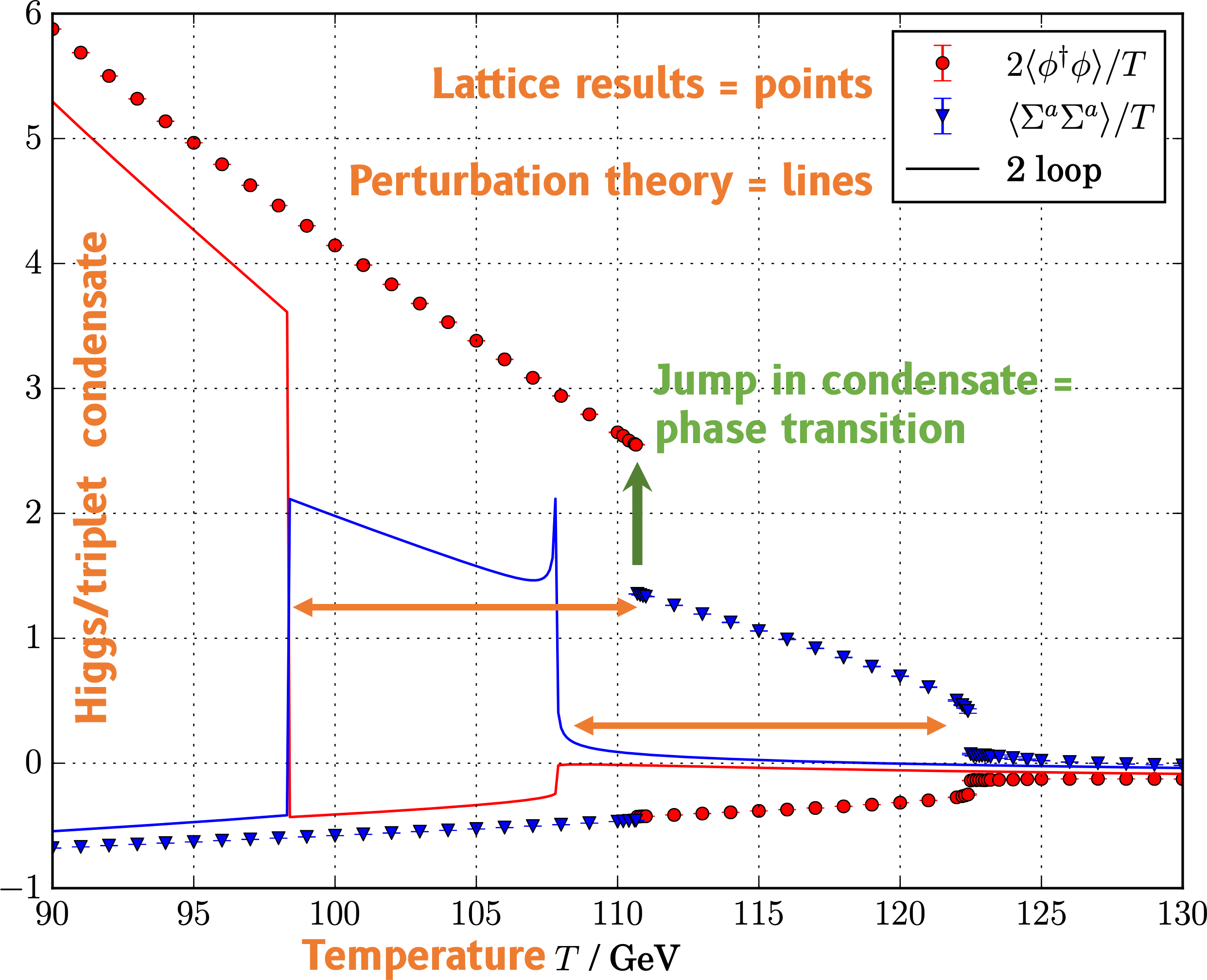
Need benchmarks: perturbation theory out by $\gtrsim 10\%$
Intro to EPWT - conclusion
- SM is a crossover
- Many simple extensions with first order phase transitions
- Will take a next-generation collider (or GW detection/exclusion!) to rule out most models
- And need new Monte Carlo simulations to benchmark perturbation theory studies
Why do we need simulations?
A toy model example.
Toy model of a real scalar field
Let us explore how all this machinery works for the scalar field $\phi$, with Lagrangian $$ \begin{align} \mathcal{L} & = \frac{1}{2} (\partial_\mu \phi)^2 - V(\phi) \\ V(\phi) & = \sigma \phi + \frac{1}{2}m^2 \phi^2 + \frac{1}{3!}g \phi^3 + \frac{1}{4!} \lambda \phi^4 \end{align}$$ and neglect couplings to other fields for simplicity.
(If we coupled it to the Standard Model, could be a DM candidate for example)
Infrared problem
- At low temperatures the perturbative expansion parameter is $\lambda$...
- ...so at high temperatures it will be of the form $\frac{\lambda T}{m}$, with $m$ the mass of some bosonic excitation.
- But the field undergoing the phase transition is often light compared to the temperature $T$.
- Thus $T/m \gg 1$ and the expansion is poorly behaved.
Aside: pure gauge theory
- Furthermore gauge bosons are perturbatively massless at high temperatures (in their symmetric phase)
- If we want to study (de)confinement phase transitions, then lattice methods are essential
- We studied bubble nucleation for the first time recently in $\mathrm{SU}(8)$, see arXiv:2603.22088 .
3D effective field theory
- As mentioned above, the field becomes light close to the phase transition, due to cancellations between tree-level and thermal contributions.
- Then the expansion parameter $\lambda T/m$ can become large, and perturbation theory breaks down.
- The solution is high-temperature dimensional reduction: one writes down a 3D effective field theory with only the light fields.
3D model
Let us consider the following theory in three Euclidean dimensions (which happens to be the most general theory with the same symmetries and number of fields): $$ \begin{align} \mathcal{L}_3 & = \frac{1}{2} (\partial_i \phi_3)^2 - V_3(\phi_3) \\ V_3(\phi_3) & = \sigma_3 \phi_3 + \frac{1}{2}m_3^2 \phi_3^2 + \frac{1}{3!}g_3 \phi^3 + \frac{1}{4!} \lambda_3 \phi_3^4 \end{align}.$$ This is interesting in itself, but is also a high-temperature effective field theory for our 4D model.
Dimensional reduction
How do we match the 4D model (possibly the whole Standard Model with extra field content) to the 3D effective field theory?
- Having written down the most general 3D model with all the light degrees of freedom, we:
- Compute correlation functions in the 4D and 3D theories
- Compare the results of the two theories for momenta $p\sim \sqrt{\lambda} T$
- Use these results determine the relationship between the 4D and 3D couplings
'generic rules' paper: hep-ph/9508379
Lattice model
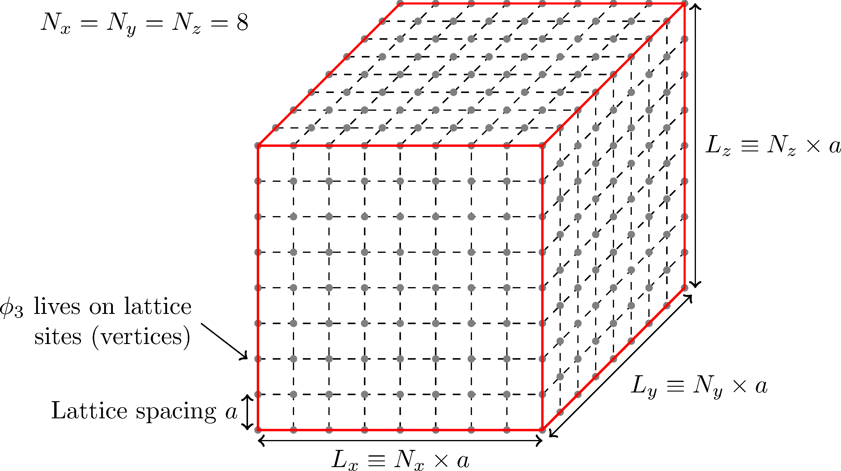
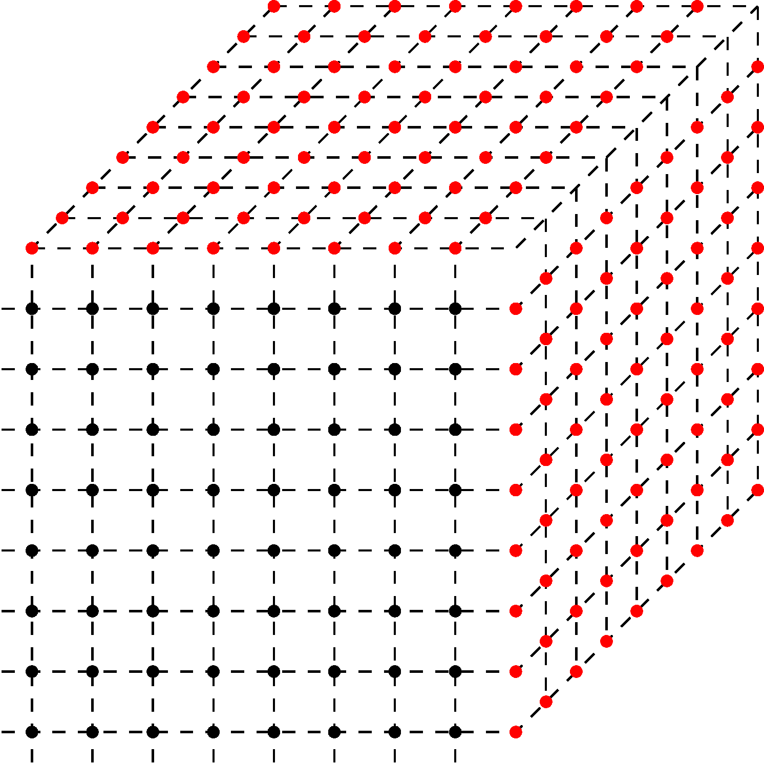
We can discretise our three-dimensional effective field theory with Euclidean Lagrangian $$ \mathcal{L}_{3,\text{lat}}(\mathbf{x}) = \frac{1}{2a^2} \sum_{i} \left[\phi_3(\mathbf{x} + \hat{\imath}) - \phi_3(\mathbf{x})\right]^2 + V_{3,\text{lat}}[\phi_3(\mathbf{x})] $$ where $$ \begin{multline} V_{3,\text{lat}}[\phi_3(\mathbf{x})] \\ = \sigma_{3,\text{lat}} \phi_3(\mathbf{x}) + \frac{1}{2} m_{3,\text{lat}}^2 \phi_3(\mathbf{x})^2 + \frac{1}{3!} g_3 \phi_3(\mathbf{x})^3 + \frac{1}{4!} \lambda_3 \phi_3 (\mathbf(x))^4 \end{multline} $$ (soon you will play with a code that implements this)
Lattice setup
- Physical size $V \equiv L_x \times L_y \times L_z$
- Number of sites $N_x \times N_y \times N_z$
- Lattice spacing $a$
Infinite volume limit
- As well as taking $a \to 0$ we need to extrapolate to infinite volume $V \to \infty$, with $L_x, L_y, L_z \to \infty$.
- Ideally:
- Fix $a$ and extrapolate $V\to \infty$.
- Then vary $a$ and extrapolate again.
- Then extrapolate $a \to 0$.
- Often it is enough to vary $a$ at some fixed volume $V$ to check the dependence on lattice spacing is not too strong.
Periodic boundary conditions
Physics is translation-invariant, so usually impose periodic boundary conditions
Lattice-continuum relations and continuum limit
How do we match the 3D continuum to the 3D lattice model?
- Compute the effective potential in continuum and on the lattice.
- Equate the two, in $\overline{MS}$ for continuum, and for finite lattice spacing $a$ on the lattice.
- Ensures that the lattice theory converges to the continuum theory as $a\to 0$.
- We then need to extrapolate simulation results to the continuum ($a\to 0$) as well.
What parameters do we choose?
- Having picked 4D parameters, we match them to our 3D EFT parameters, and then relate them to the lattice parameters with the lattice-continuum relation.
- The 4D to 3D mapping is not one-to-one because we integrate out a lot of field content, can thus sometimes recycle simulations
- Then need to extrapolate to zero lattice spacing $a\to 0$, and infinite volume $V \to \infty$
Monte Carlo - importance sampling
- We want to measure quantities like $\langle \phi \rangle$ on the lattice, i.e. evaluate $$ \langle \phi \rangle = \frac{1}{Z} \int \mathcal{D} \phi \; \phi \, e^{-S_\text{lat}}; \quad S_\text{lat} = \sum_\mathbf{x} \mathcal{L}_{3,\text{lat}}(\mathbf{x}) $$
- Very high-dimensional integral, $L_x \times L_y \times L_z$ points, each with its own value of $\phi$.
- But this integral is peaked around the extremum of the exponent - use importance sampling.
Monte Carlo - measurements
- Generate lattice configurations $i$ with probability weighted by $e^{-S_\text{lat}}/Z$.
- Then $ \langle \phi \rangle $ is just a sum over measurements with configuration, $ \langle \phi \rangle = \sum_i \phi_i $.
- $Z$ cannot be measured directly, so we only know relative probability of configurations.
Metropolis algorithm
- Markov Chain: generate next configuration from current configuration, no memory (e.g. vary $\phi$ at one site by a random amount)
- Calculate change in Euclidean action $\Delta S_\text{lat}$.
- Nicholas Metropolis, Arianna W. Rosenbluth, Marshall Rosenbluth, Augusta H. Teller and Edward Teller (1953): accept next configuration with probability $$ W = \text{min} (1, e^{-\Delta S_\text{lat}}).$$
What do the histograms look like?
At the critical coupling, the probability density between the phases falls exponentially with volume:
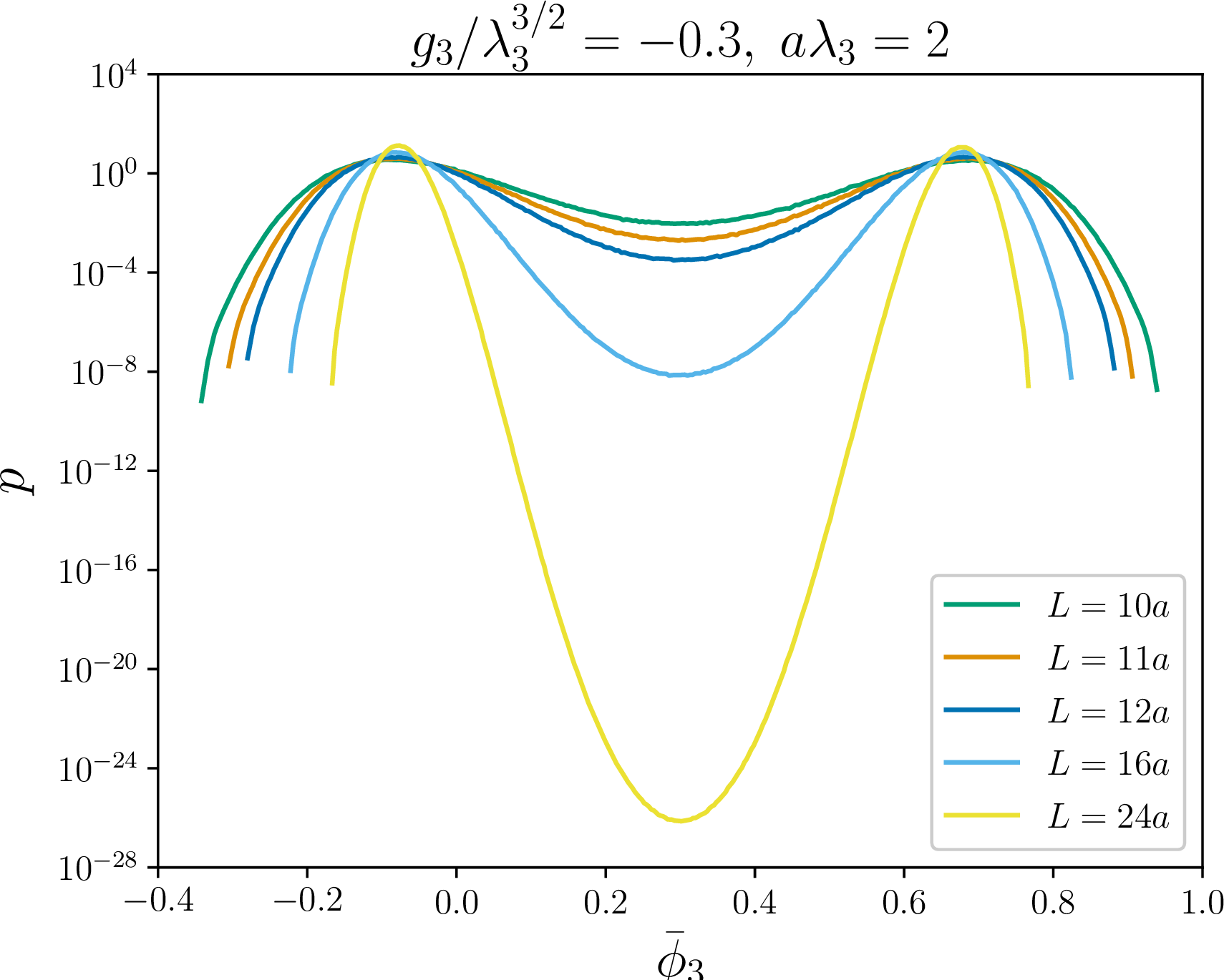
From arXiv:2101.05528
Reweighting
- If we simulate with one set of parameters we can reweight our results to 'nearby' parameters, so long as we keep track of the corresponding term in the action:
- Suppose we want to reweight in $m_3^2$ to $m_3'^2$.
- It enters into the action as $$ S \supset \frac{1}{2}m_3^2 \sum_\mathbf{x} \phi_3(\mathbf{x})^2 \equiv \frac{1}{2}m_3^2 \theta.$$
- We need to record $\theta$ during our simulation, as well as what we want to observe $\mathcal{O}$.
- $\theta$ and $\mathcal{O}$ might be the same!
The reweighting formula
- We have (for $N$ measurements labelled $i$) $$ \left< \mathcal{O} \right>_{m_3'^2} = \frac{ \sum_{i=1}^N \mathcal{O}_i e^{-\frac{1}{2}(m_3'^2 - m_3^2)\theta_i }}{\sum_{i=1}^N e^{-\frac{1}{2}(m_3'^2 - m_3^2)\theta_i }} $$
- A bit like Bayes' theorem.
- Concept is due to Alan Ferrenberg and Robert Swendsen, Phys. Rev. Lett. 61 (1988) 2635.
What does reweighting look like?

From hep-lat/0103036
Multicanonical simulations
- When the barrier is too high, the Monte Carlo simulation will not tunnel at all
- Then use the multicanonical method:
- Use a modified Boltzmann weight in Monte Carlo, $ p_\text{muca} \sim e^{-S_\text{lat} + W(\theta)} $
- Here, $W(\theta)$ is a weight function parameterised by e.g. order parameter $\theta$ that enhances tunnelling
Running a multicanonical simulation
- Ideally choose $W(\theta) = -\log p_\text{can}(\theta)$, where $p_\text{can}(\theta)$ is the canonical ensemble probability
- Then, $p_\text{muca}$ would be flat by construction!
- We don't know $p_\text{can}$ (because the simulation would take too long to tunnel) so we have to build $W(\theta)$ iteratively.
Further reading on the analytical theory stuff
- Basics of Thermal Field Theory by Mikko Laine and Aleksi Vuorinen forms a great textbook.
- Section 6 (pp 86-87) is most relevant.
- Our toy model is extensively discussed by Oliver Gould in arxiv:2101.05528.
- The classic paper on dimensional reduction is the so-called 'generic rules' paper, hep-ph/9508379.
- And the first paper to put everything together with simulations was perhaps hep-lat/9510020.
Further (pedagogical) resources on simulations for phase transitions
- Kari Rummukainen's slides and lecture notes.
- Jarno Rantaharju's (related) notes.
- Often field theory simulation textbooks are focussed on either lattice QCD or condensed matter. Our subject is in between.
- Here are two choices from the 'QCD' side of things:
- Quantum Fields on a Lattice by István Montvay and Gernot Münster
- Lattice Gauge Theories: An introduction by Heinz Rothe (open access)
Workshop section
You can find the demos at github.com/davidjamesweir/2026-lecture-demos

Tomorrow
- Extracting key equilibrium quantities from simulations
- Nucleation rate
Feel free to leave questions and feedback on Presemo!
presemo.helsinki.fi/weir
Day 2
From lattice simulations to cosmology via nucleation
'Histogram method'
First proposed by Kurt Binder in early 1980s; basic quantity is the distribution of the order parameter:

Critical point
- Critical couplings = equal peaks
- Once we have determined the critical coupling we can use the machinery we discussed yesterday to get the critical temperature:
- Lattice-continuum relations give us the continuum 3D critical couplings
- Matching relations give us 4D critical couplings
- Matching can be non-unique, but if we fix the 4D couplings and vary the temperature, we can usually match to the 3D theory
Relating lattice results to 4D physics
- Often good to determine the 'trajectory' in 3D parameter space as a function of $T$ beforehand.
- Fix $4D$ parameters $\sigma, m^2, g, \lambda$.
- Determine matching relations for continuum 3D parameters $\sigma_3, m_3^2, g_3, \lambda_3$ as a function of $T$.
- Also useful to have the partial derivatives with respect to $T$ (as we will see): $$ m_3^2(T) = f(T | \sigma, m^2, g, \lambda); \quad \frac{\partial m_3^2}{\partial T} = \frac{\partial f}{\partial T}. $$
- May need to reweight lattice results in more than one parameter to vary $T$.
For concreteness:
Recalling: $$ V_3(\phi_3) = \sigma_3 \phi_3 + \frac{1}{2}m_3^2 \phi_3^2 + \frac{1}{3!}g_3 \phi^3 + \frac{1}{4!} \lambda_3 \phi_3^4 $$ the matching relations at leading order in our theory are $$\begin{align} \sigma_3(T) & = \frac{\sigma}{\sqrt{T}} + \frac{g T^{3/2}}{24} \\ m_3^2 (T) & = m^2 + \frac{\lambda T^2}{24} \\ g_3(T) & = \sqrt{T}g \\ \lambda_3 (T) & = T \lambda \\ \end{align} $$
From arXiv:2101.05528 appendix.
From histograms to free energies
- We associate the probability $P(\theta)$ of observing a given order parameter $\theta$ with a constrained free energy $F(\theta)$, such that $P(\theta) \propto e^{-F(\theta)}$.
- We can't measure $Z$, since we are doing importance sampling; only know relative probabilities $P(\theta)$.
- From our histogram ($\equiv$ estimate of the probability distribution of $\theta$), can read off free energy differences: $$F(\theta) = \log P(\theta) + \text{constant}$$ (personally think this defines constrained free energy)
Another justification of the constrained free energy
This comes from James Langer's paper,
Metastable states Physica 73 (1974) 61-72.
$$ e^{-F(\theta)} = \sum_{\substack{\text{(constrained microscopic } \\ \text{variables with $\theta$ fixed)}}} e^{-H}$$ where $H$ is a Hamiltonian
describing the short-range physics.
See arXiv:2108.04377 for a modern discussion in the context of bubble nucleation.
What do we want?
We need to know the following to study the out-of-equilibrium dynamics of the phase transition
(including gravitational waves):
- Critical temperature [done]
- Surface tension [next]
- Latent heat/phase transition strength
- Nucleation rate, and hence nucleation temperature
- Wall velocity [later on]
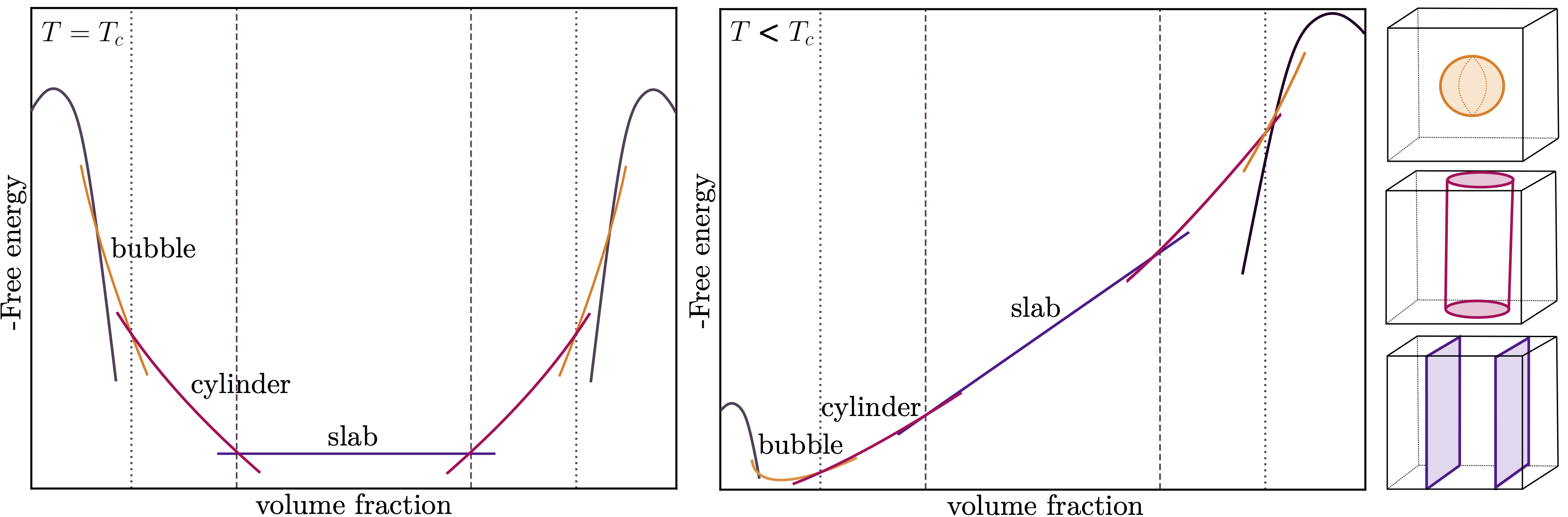
Thin wall approximation
- Consider a cubic lattice for simplicity.
- Suppose our lattice contains a mixed configuration of two phases.
- Assume the phase boundary is well-localised compared with the lattice size.
- Energy per unit area of the phase boundary is the surface tension $\sigma$.
- For any given value of the order parameter $\theta$, the favoured mixed configuration will be that which minimises the free energy.
Free energy at the critical temperature

From From hep-lat/0103036
The surface tension $\sigma$
- This is the free energy per unit area of the interface between the the two phases.
- The transverse fluctuations of the interface are proportional in size to $\sqrt{T/\sigma}$.
- Only defined at phase coexistence, i.e. critical temperature.
- Can be used to estimate the action of a critical bubble in the thin-wall limit, and hence estimate nucleation rate.
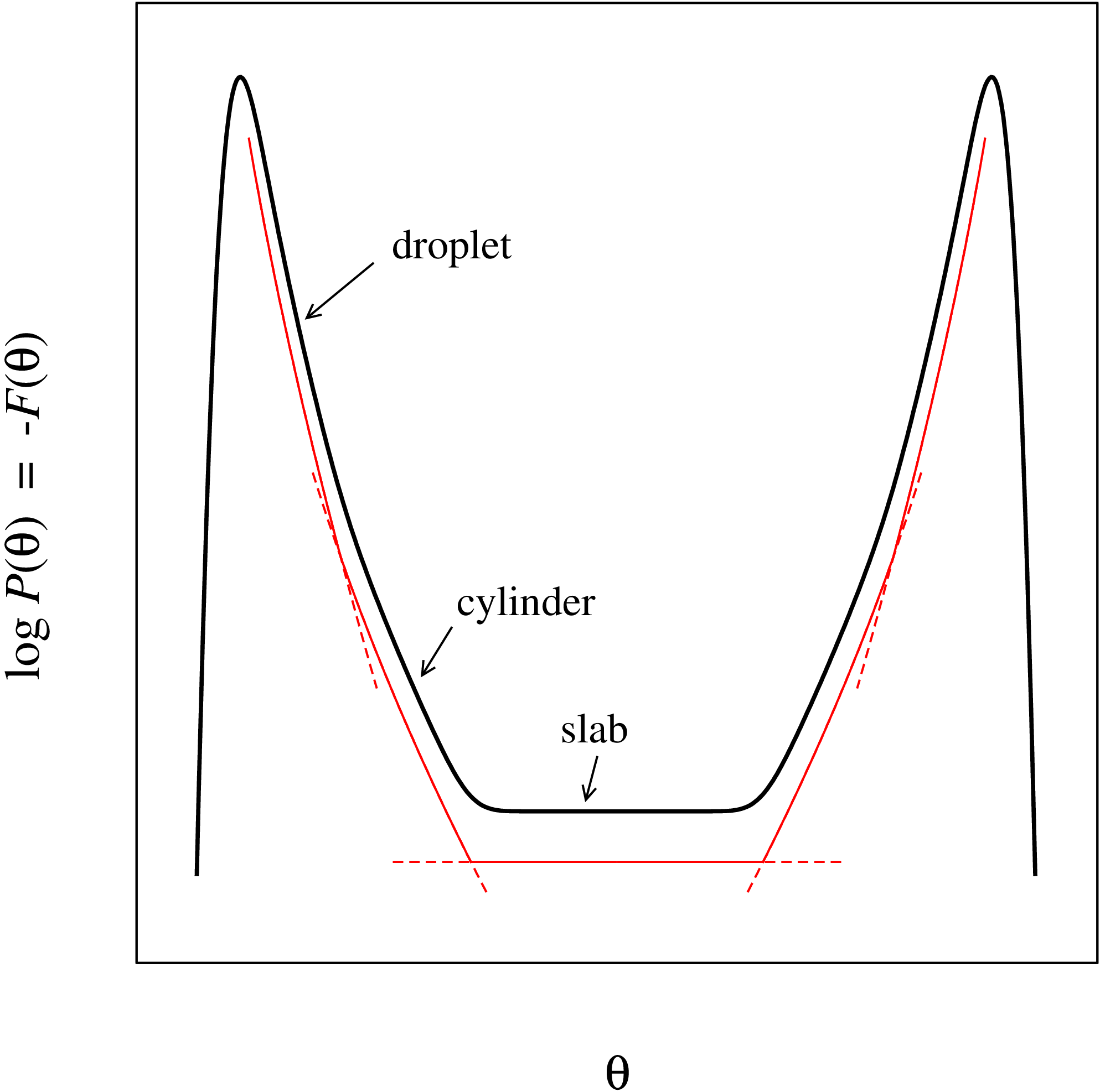
Measuring the surface tension $\sigma$
- Must be the slab interface so we know its area
$\Rightarrow$ can use non-cubic geometries to help. - Then (neglecting fluctuations and finite size effects) $$ \sigma = -\lim_{V\to\infty} \frac{1}{2L_x L_y} \log \frac{P_\text{slab}}{P_\text{peak}} $$ (factor 2 because two boundaries)
- $P_\text{slab}$ is the bottom of the histogram, corresponding to slab geometry.
- Now we can see that $P_\text{slab}/P_\text{peak} \sim e^{-2 \sigma L_x L_y}$, so indeed goes down exponentially with volume.
The latent heat $L$
- This is the difference in enthalpy between the two phases.
- Again, only defined at phase coexistence.
- (Below the critical temperature, the energy released by a phase transition is not just $L$, but also some free energy.)
Measuring the latent heat $L$
By definition (from the Clapeyron equation), $$ \frac{L}{T} = \left. \frac{\mathrm{d} \Delta p}{\mathrm{d} T} \right|_{T_c} = \frac{T}{V} \left[\frac{\mathrm{d}}{\mathrm{d}T}\Delta \log Z\right]_{T_c} = \frac{T}{V} \frac{\mathrm{d}}{\mathrm{d}T} \Delta P, $$
- $\Delta p$ is the pressure difference between the two phases.
- We treat the two phases as having separate subsystem partition functions so we can measure $\Delta \log Z$.
- $\Delta F \equiv - T \Delta \log Z$ is the free energy difference between the phases. We infer $\Delta F/V = \Delta p $ at coexistence.
- And $\Delta P$ is the difference in probabilities under the two peaks.
There is another way!
- Starting from the free energy density $\Delta f$, can write down another version of the Clapeyron equation $$ L = - \frac{\partial \Delta f}{\partial T}; \qquad \Delta f \equiv T \Delta \varepsilon_\text{vac} $$ where $\Delta \varepsilon_\text{vac}$ is the 3D vacuum energy.
- Derivatives with respect to $T$ only enter this through the couplings in the potential energy, so $$ \frac{L}{T} = \ldots + \frac{1}{2} \frac{\partial m_3^2}{\partial \log T}\Delta \langle \phi_3^2 \rangle + \ldots. $$
- Bigger condensate jump $\Rightarrow$ stronger transition!
This approach is lucidly explained e.g. in arXiv:2101.05528, section 3.2.
Determining the nucleation rate
Now we know the critical temperature, surface tension, and latent heat, what about nucleation?
Motivation
- Basic goal: calculate probability of a bubble of new phase appearing in the old phase
- Details depend somewhat on temperature:
- At zero temperature - quantum process
- At high temperature - thermal process
- Rate of nucleation important for determining whether phase transition will complete
- Nucleation rate a key factor in determining GW power spectrum amplitude
Further reading
- Basic idea: James Langer
- Quantum nucleation: Sidney Coleman; Curtis Callan and Sidney Coleman
- At nonzero temperature: Andrei Linde
- The nonperturbative approach: Guy Moore and Kari Rummukainen
Nucleation basics
- When the universe drops below the critical temperature, broken phase is the new global minimum.
- Quantum (or thermal) fluctuations will excite the field across the potential barrier to the new minimum.
- Consider a single scalar field $\phi$ with Lagrangian $$ \mathcal{L} = \frac{1}{2} \partial_\mu \phi \partial^\mu \phi - U(\phi) $$ and equation of motion $$ \frac{\partial^2 \phi}{\partial t^2} + \nabla^2 \phi = U'(\phi).$$
More nucleation basics
- Want to calculate probability for field $\phi$ to tunnel from false vacuum $\phi_+$ to true vacuum $\phi_-$.
- Like quantum mechanical tunnelling.
- Solve for trajectory that 'bounces' from $\phi_+$ to $\phi_-$ and back again in a localised region
- Obtain exponential factor $B$ in nucleation rate $\Gamma/V \propto Ae^{-B}$.
A bit more about Langer's theory
- Langer's theory puts this on a rigorous footing.
- The rate is the integral of the probability flux $J$ over the transition surface in free energy, $\Gamma = \int_S J \cdot \mathrm{d}S_\perp$
![]() figure from arXiv:2108.04377.
figure from arXiv:2108.04377.
- Recently tested directly in arXiv:2505.22732.
Computing the bounce
- Coleman: work in imaginary time $t \to it$, and extremise the resulting Euclidean action.
- At $T=0$, system has $\mathrm{O}(4)$ invariance: $$ \frac{\mathrm{d}^2 \phi}{\mathrm{d} \rho^2} + \frac{3}{\rho} \frac{\mathrm{d} \phi}{\mathrm{d} \rho} = U'(\phi); \qquad \rho = \sqrt{t^2 + \mathbf{x}^2}$$ with boundary conditions $$ \lim_{\rho \to \infty} \phi(\rho) = \phi_+ ; \qquad \left. \frac{\partial \phi}{\partial_\rho} \right|_{\rho=0} =0 $$
- Solve and then compute the action $S_4$ for this path.
Fluctuations and finite temperature
- Prefactor given by the fluctuations about the bounce path.
- However, we are interested in the finite-$T$ version of this calculation, in which case the symmetry is $\mathrm{O}(3)$.
- Use dimensional analysis to guess the prefactor: $$ \frac{\Gamma}{V} \approx T^4 \exp \left( -\frac{S_3(T)}{T} \right) $$ with $$ S_3 = 4\pi \int \mathrm{d}r \, r^2 \left[ \frac{1}{2} \left( \frac{d \phi}{d r} \right)^2 + V_\text{eff}(\phi, T) \right]. $$
Nucleation rates
- The full (finite-T) expression is $$ \begin{multline}\frac{\Gamma}{V} = \frac{\omega_-}{\pi} \left(\frac{S_3}{2\pi T} \right)^{3/2} \left[ \frac{\mathrm{det'}\left[ -\nabla^2 + V''(\phi_-, T)\right]}{\mathrm{det} \left[ -\nabla^2 + V''(\phi_+,T)\right] } \right]^{-1/2} \\ \times \exp \left( - \frac{S_3(T)}{T} \right). \end{multline} $$
- The above expression is very similar to that for the sphaleron rate - the two processes have much in common
Limiting cases for $S_3$
- As discussed above, solve for bounce profile by shooting.
- Identify two limiting cases depending on nucleation temperature $T_N$
- For small supercooling ($T_\mathrm{c} - T_N \ll T_\mathrm{c}$), bubbles are thin-wall type (with $\tanh$ walls).
- For large supercooling $T_N \ll T_\mathrm{c}$, bubbles are close to a Gaussian.
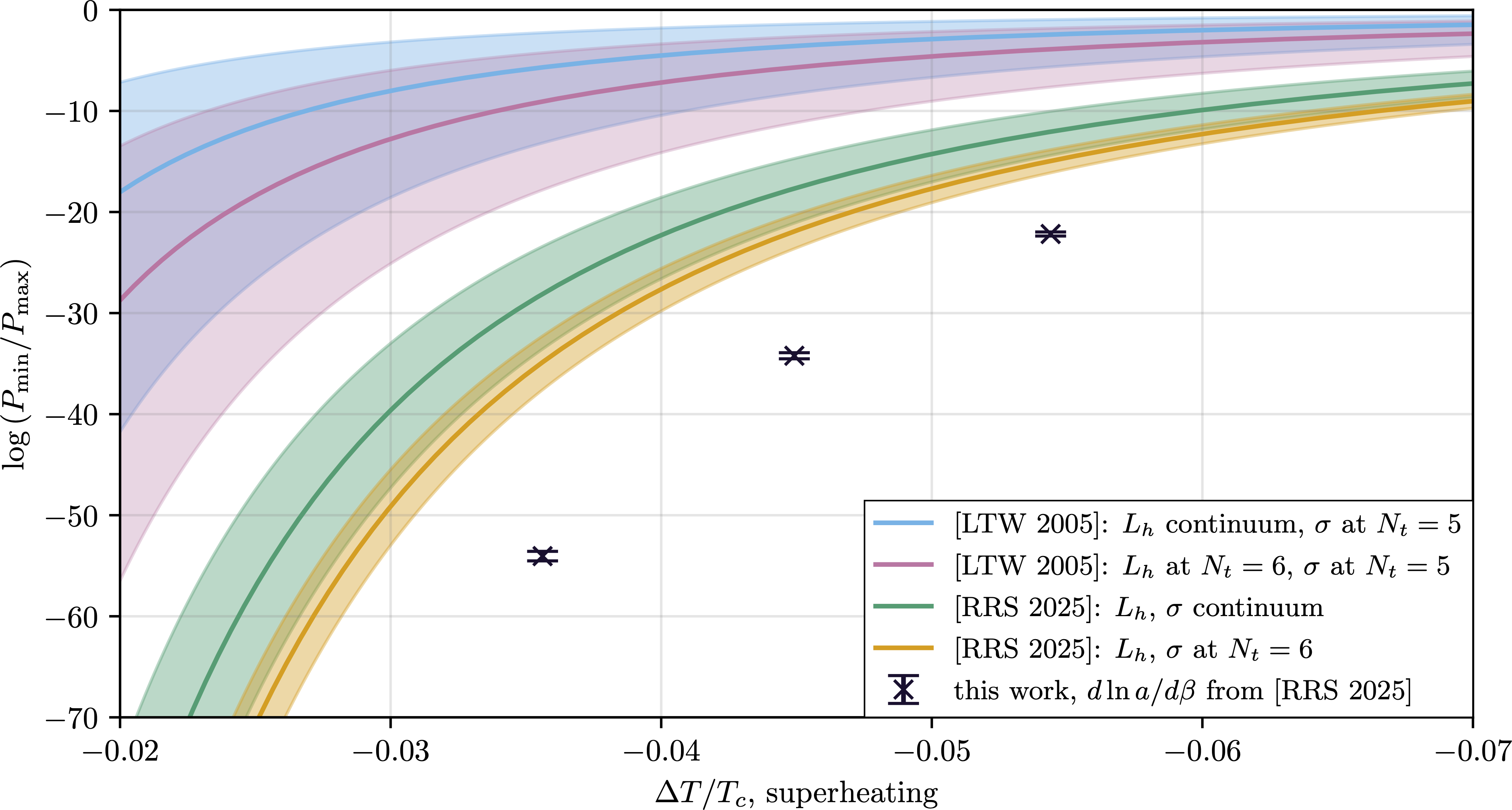
From thin to thick walls
Thin-wall with lattice data
PRD 37 (1988) 1380; see also hep-ph/0009132 section V A
- Bubble radius is much thicker than the phase boundary thickness, so treat the surface as a thin wall.
- Surface tension $\sigma$ at the nucleation temperature $T_N$ is the same as at the critical temperature $T_c$.
- Expanding the Clapeyron relation $\frac{L}{T} = \frac{\mathrm{d} \Delta p}{\mathrm{d} T}$ for small $\Delta T = T_N -T_c$, pressure difference is related to the latent heat (measured at the critical temperature) by $$\Delta p = L (T_N - T_c)/T_c$$
Thin-wall with lattice data
- Then the action of a bubble of radius $r$ is $$ \begin{align} S_3(r) & = 4\pi r^2 \sigma - \frac{4\pi}{3} \Delta p r^3 \\ & = 4\pi r^2 \sigma - L\frac{(T - T_c)}{T_c} r^3 \end{align} $$
- Extremising over $r$, we find $$ \frac{\mathrm{d} S_3}{\mathrm{d} r} = 0$$ $$ \Rightarrow r = \frac{2 \sigma }{\Delta p}, \quad S_3 = \frac{16\pi \sigma^3}{3 (\Delta p)^2} = \frac{16\pi \sigma^3 T^2}{3 L^2 (T - T_c)^2} $$
Thin-wall with lattice data
- We can then plug $S_3 = \frac{16\pi \sigma^3 T^2}{3 L^2 (T - T_c)^2}$ into the rate ansatz, $$ \frac{\Gamma}{V} \approx T^4 \exp \left(- \frac{16\pi}{3} \frac{\sigma^3 T}{L^2 (T - T_c)^2} \right) $$
- Can use this for any theory for which we can measure surface tension and latent heat.
- This includes strongly coupled theories (see e.g. arXiv:2603.22088), but
- Still thin-wall
- Only strictly valid at small supercooling
Aside: $\mathrm{SU}(8)$ example
From arXiv:2603.22088
Beyond $S_3$
- Using $S_3(T)/T$ as the exponential parameter in the nucleation rate is a high-temperature approximation.
- One can also compute the nucleation rate
nonperturbatively, both the prefactor and the
exponential part. Results suggest that (for SM):
- True supercooling lies between 1- and 2-loop results
- 2-loop perturbative surface tension close to true result
- See recent updated results in arXiv:2205.07238
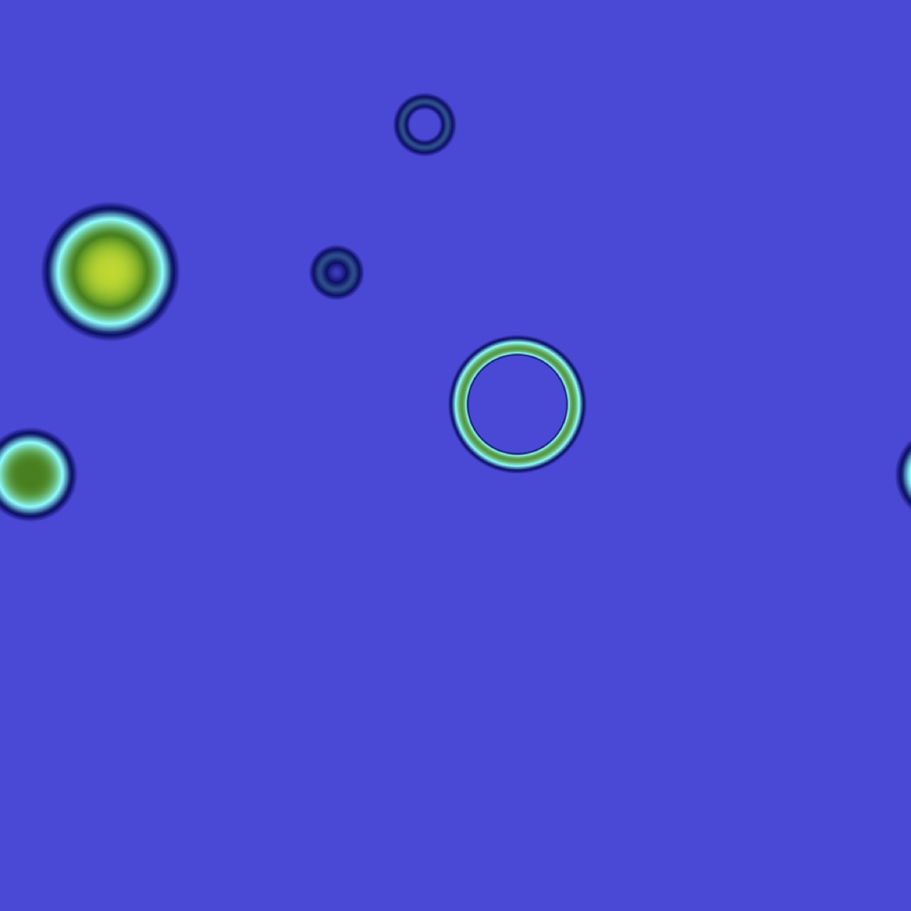
Bubble nucleation, nonperturbatively
Free energy below $T_c$
Adapted from figure by Riikka Seppä, arXiv:2603.22088
If we can generate 'bubble' configurations in a Monte Carlo simulation, we can use them as the starting point to measure the nucleation rate nonperturbatively.
Bubble nucleation rate on the lattice
General idea is that the nucleation rate is a product of:
- Relative probability (density) of critical bubbles, $P_c$
- Rate of change of the order parameter with time for a bubble being nucleated, the 'flux'
- Number of times a critical bubble tunnels back and forth before settling back to one or the other phase, $\mathbf{d}$
Then $$\Gamma V = P_c \left< \frac{1}{2}\text{flux} \times \mathbf{d} \right> \approx P_c \frac{1}{2} \left< \text{flux} \right> \left< \mathbf{d} \right>.$$
Probability of critical bubbles
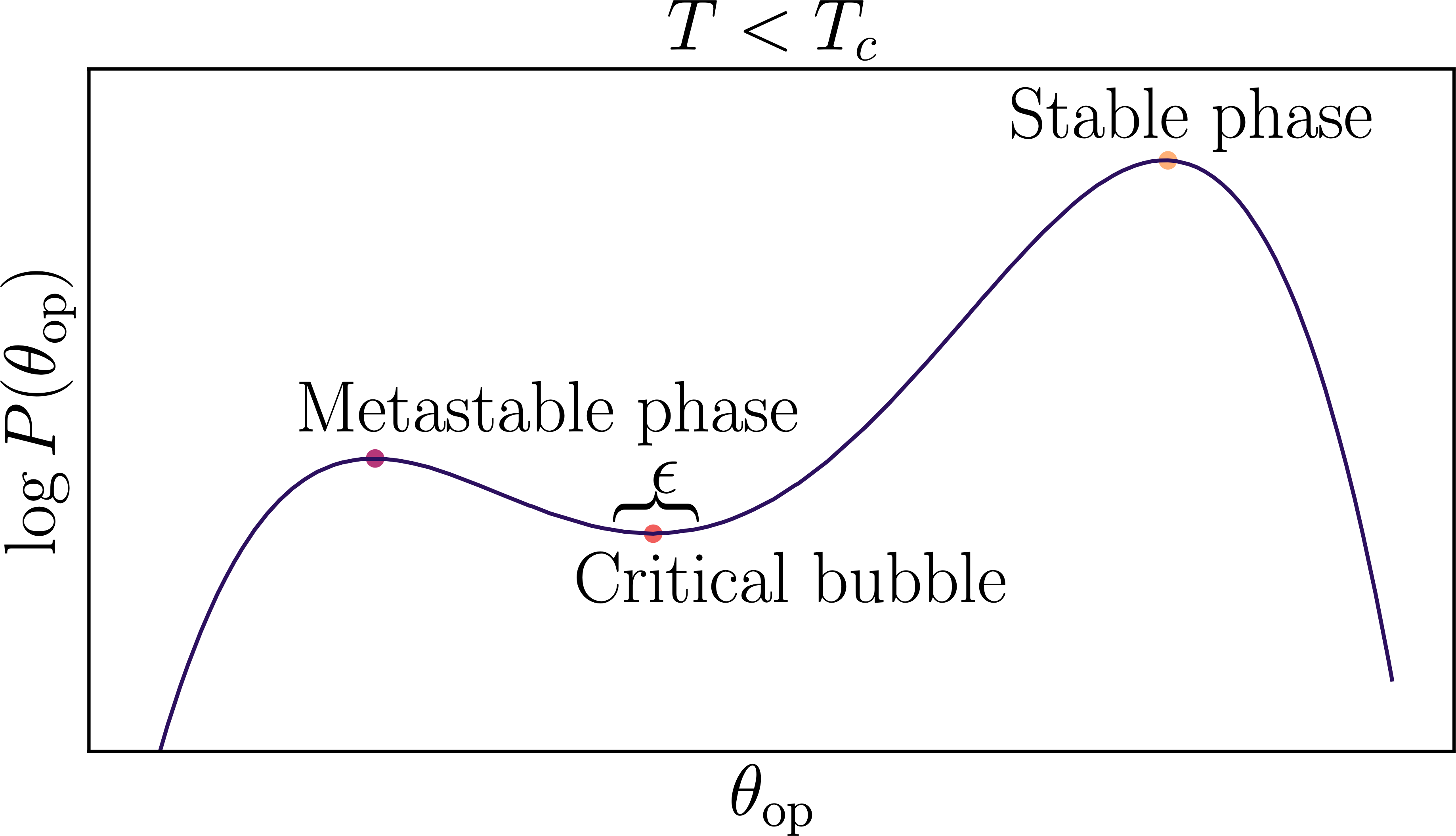
Probability density of a configuration lying in $\varepsilon$ relative to being in the metastable phase: $$ P_c = \frac{P(|\theta - \theta_c| < \varepsilon/2)}{\varepsilon P(\theta < \theta_c)}.$$
Generating critical bubbles
- Critical bubble configurations are heavily suppressed, and we need large volumes to see them:
- Use multicanonical simulations so critical bubbles are not suppressed.
- Save configurations that lie in the region $\varepsilon$.
Do those bubbles tunnel?
- Given the candidate critical configurations, evolve them with the equations of motion in a heat bath backwards and forwards in time.
- If they tunnel, then $\mathbf{d} = 1/N_\text{crossings}$, otherwise $\mathbf{d} = 0$.
Created by Anna Kormu, arXiv:2404.01876
What do trajectories look like?
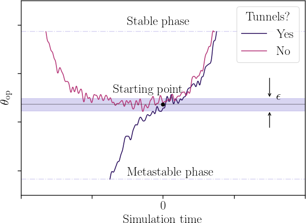
Credit: Anna Kormu
Assembling the rate
- Rate is
$$\Gamma V = P_c \left< \frac{1}{2}\text{flux} \times \mathbf{d} \right> \approx P_c \frac{1}{2} \left< \text{flux} \right> \left< \mathbf{d} \right>.$$
- Get $P_c$ from histogram.
- Get $\langle \mathbf{d} \rangle$ from real time evolution of candidate critical bubbles.
- And $\langle \text{flux} \rangle$ can be calculated analytically
(see e.g. hep-lat/0103036).
Nucleation rate on the lattice
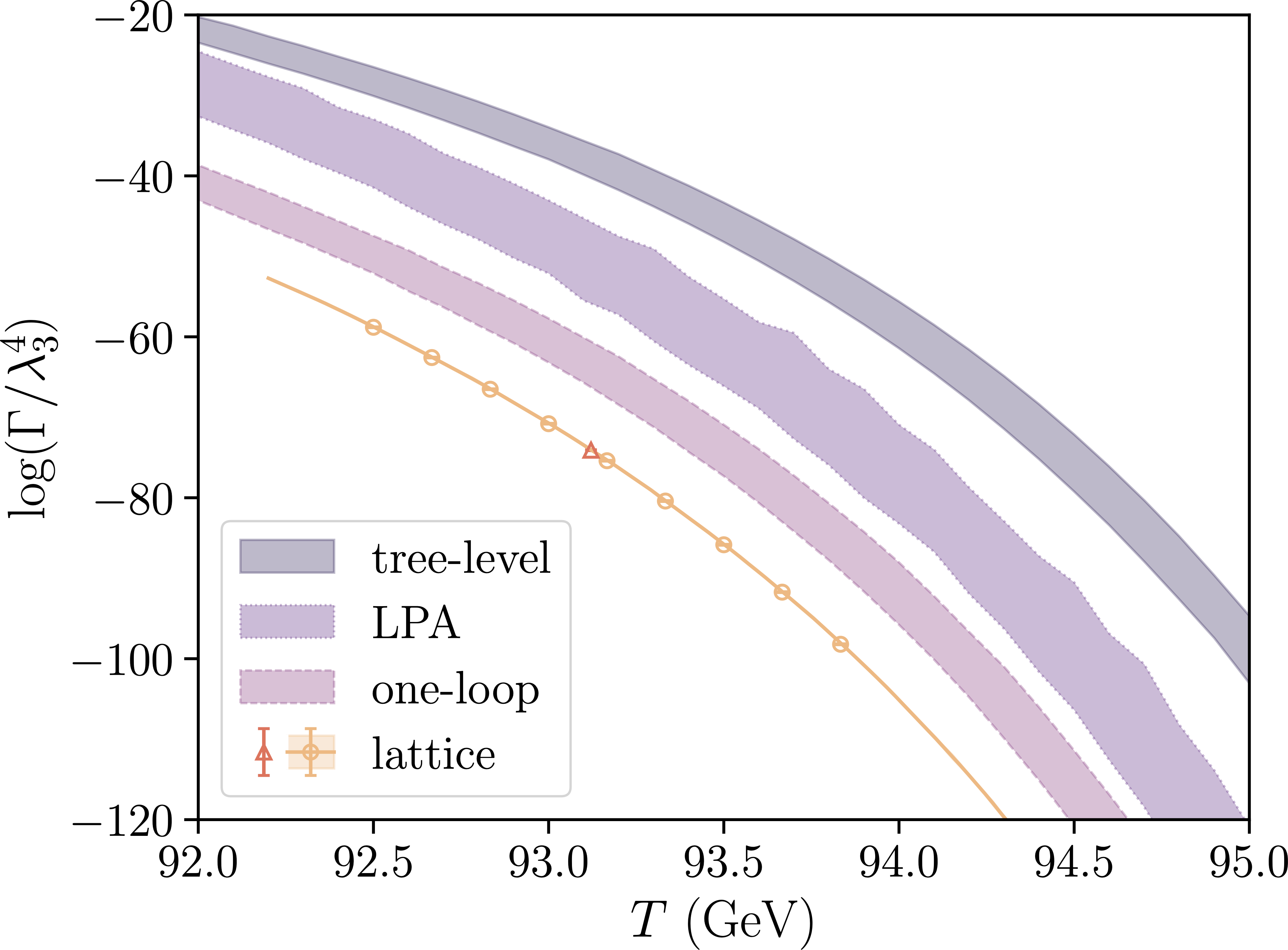
From arXiv:2404.01876.
Making use of $\Gamma$
- The nucleation rate $\Gamma$ gives the probability of nucleating a bubble per unit volume per unit time.
- More useful for cosmology is to consider the inverse duration of the phase transition, defined as $$ \beta \equiv - \left.\frac{d S(t)}{d t} \right|_{t=t_*} \approx \frac{\dot \Gamma}{\Gamma} $$
- Phase transition completes when the probability of nucleating one bubble per horizon volume is order 1 $$ S_3(T_*)/T_* \sim -4 \log \frac{T_*}{m_\mathrm{Pl}} \approx 100 $$
Making further use of $\Gamma$
- Using the adiabaticity of the expansion of the universe the time-temperature relation is $$ \frac{d T}{d t} = - T H $$
- This gives, for the ratio of the inverse phase transition duration relative to the Hubble rate, $$ \frac{\beta}{H_*} = T_* \left. \frac{dS}{dT} \right|_{T = T_*} = T_* \frac{d}{d T} \left. \frac{S_3(T)}{T} \right|_{T=T_*}$$
- If $\frac{\beta}{H_*} \lesssim 1$ then the phase transition won't complete...
Nucleation - conclusion
- Rate per unit volume per unit time $\Gamma$ computed from bounce actions $S(T) = \mathrm{min}\{S_3(T)/T ,S_4(T) \}$
- Inverse duration relative to Hubble rate $\frac{\beta}{H_*}$ computed from $\Gamma$, and controls GW signal
- To get $\beta$:
- Find effective potential $V_\text{eff}(\phi,T)$
- Compute $S_3(T)/T$ (or $S_4(T)$) for extremal bubble by solving 'equation of motion'
- Determine transition temperature $T_*$
- Evaluate $\beta/H$ at $T_*$
- Use $\beta/H_*$ as input to compute GWs (c.f. $B$ earlier!)
Workshop section
- Our lattice computation of the nucleation rate used a combination of multicanonical Monte Carlo and real time simulations.
- At small enough supercooling, real time simulations are enough.
- Interest in this as a method of studying phase transitions has grown in recent years, and computers are much faster than they were in the 90s.
- Today you'll have a go at reproducing the nucleation rate from one early paper on the topic.
Workshop section
Please visit
github.com/davidjamesweir/2026-lecture-demos
and load the nucleation worksheet.
Tomorrow
- Wall velocities
- Gravitational waves recap
- Redshifting a gravitational wave source
Remember to leave questions and feedback on Presemo!
presemo.helsinki.fi/weir
Day 3
Wall velocities and GW source cosmology
Wall velocities
Motivation
- Wall velocity connects the electroweak phase
transition to the two big unknowns:
- Baryogenesis (rate of baryon asymmetry production)
- Gravitational waves ($v_\text{wall}^3$ dependence)
- [also filtering models arXiv:1912.02830]
- [Almost] at the bottom of a hierarchy of abstraction:
- Can derive friction term for higher-level simulations
- Check how valid using a single scalar field and ideal fluid really is.
Further reading
- Tomislav Prokopec and
Guy Moore: hep-ph/9503296
and hep-ph/9506475. - Selected recent papers:
- Yago Bea
et al. (holography): arXiv:2104.05708 - Local thermal equilibrium:
- Wen-Yuan Ai, Benoit Laurent, Jorinde van de Vis: arXiv:2303.10171
- Carlo Branchina, Angela Conaci, Stefania De Curtis, Luigi Delle Rose: arXiv:2504.21213
- WallGo: arXiv:2411.04970 and wallgo.readthedocs.io
- Yago Bea
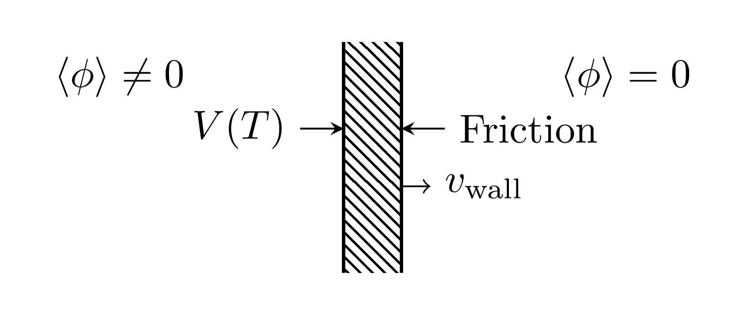
What happens at the bubble wall?
- Forces in equilibrium:
- Inside, $\langle \phi \rangle \neq 0$, latent heat $\mathcal{L} = \Delta V(T)$ released.
- Outside, $\langle \phi \rangle = 0$, friction from everything coupling to $\phi$.
- When there is no net force, wall stops accelerating.
- Is there a finite $v_\text{wall}$ below $c$ for which this happens?
- (Vacuum case: no force on wall - nothing to stop it accelerating to $c$)
- Field $\phi$ is slowly varying compared to
reciprocal momenta of particles in plasma ($\propto
T$)
⇒ treat in WKB - Write phase space density as $f(\mathbf{k},\mathbf{x})$
- Separate into equilibrium and nonequilibrium
parts, $ f(\mathbf{k},\mathbf{x}) \to f(\mathbf{k}, \mathbf{x}) + \delta
f(\mathbf{k},\mathbf{x}) $
- $f(\mathbf{k}, \mathbf{x})$ due to equilibrium thermal fluctuations; absorbed into 'finite-temperature effective potential' for $\Phi_\mathrm{cl}$
- $\delta f(\mathbf{k}, \mathbf{x})$ is the departure from that equilibrium
- Equation of motion is (schematically)
$$ \partial_\mu \partial^\mu \phi + V_\text{eff}'(\phi,T) +
\sum_{i} % \in \text{massive ds.o.f.}}
\frac{d m_i^2}{d \phi} \int
\frac{\mathrm{d}^3 k}{(2\pi)^3 2 E_i} \delta f_i(\mathbf{k},\mathbf{x}) = 0$$
- $V_\text{eff}'(\phi)$: gradient of finite-$T$ effective potential
- $f_i(k,x)$: deviation from equilibrium phase space density of $i$th species
- $m_i$: effective mass of $i$th species:
- Leptons: $m^2 = y^2 \phi^2/2$
- Gauge bosons: $m^2 = g_w^2 \phi^2/4$
- Also Higgs and pseudo-Goldstone modes
After some algebra:
$$ \overbrace{\partial_\mu T^{\mu\nu}}^\text{Force on $\phi$} - \overbrace{\int \frac{d^3 k}{(2\pi)^3} f(\mathbf{k}) F^\nu }^\text{Force on particles}= 0 $$This equation is the realisation of this idea:
Another interpretation:
$$ \overbrace{\partial_\mu T^{\mu\nu}}^\text{Field part} - \overbrace{\int \frac{d^3 k}{(2\pi)^3} f(\mathbf{k}) F^\nu }^\text{Fluid part}= 0 $$i.e.:
$$ \partial_\mu T^{\mu\nu}_\phi + \partial_\mu T^{\mu\nu}_\text{fluid} = 0 $$We will return to this later!
Layers of abstraction
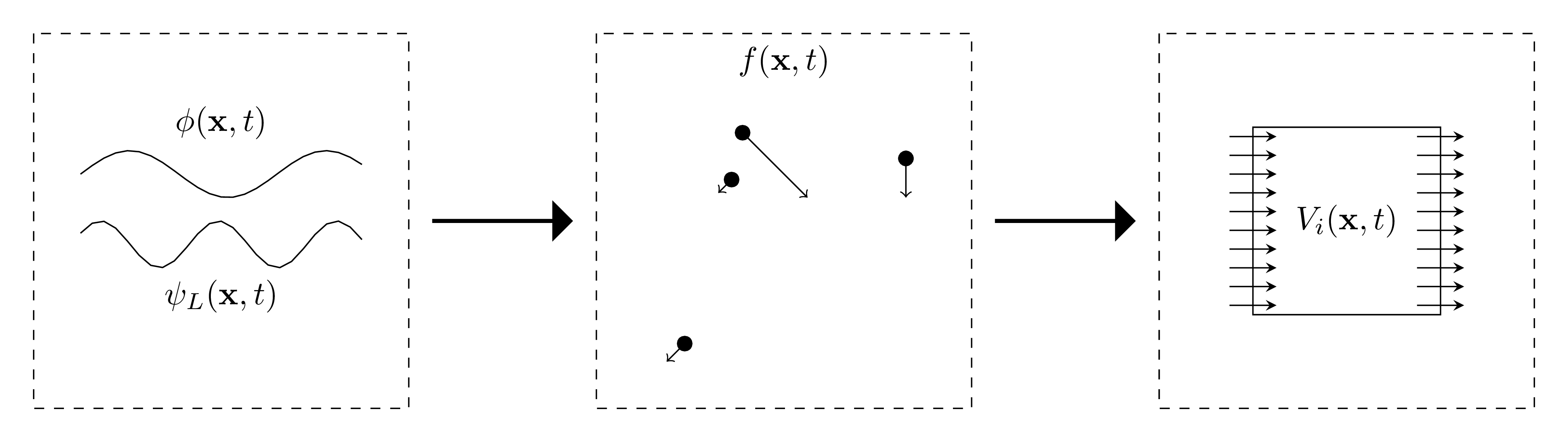
Layers of abstraction
- We have so far been using field theory equations of motion.
- Less tricky, but more abstract, are:
- Boltzmann equations
- Hydrodynamic equations
- In particular, the hydrodynamic equations we get are a valuable motivation for the rest of today's lectures
- We will now look at how to arrive at these higher-level approximations
Boltzmann equations: a reminder
What is a Boltzmann equation?
- Phase space is positions $\mathbf{x}$ and momenta $\mathbf{k}$.
- Tells us how our distribution functions $f_i(\mathbf{x},\mathbf{k})$ evolve.
- Consists of four parts:
- Time evolution $\partial_t f_i(\mathbf{x},\mathbf{k}).$
- Streaming terms in momentum and position space $\dot{\mathbf{x}} \cdot \nabla_\mathbf{x} f + \dot{\mathbf{p}} \cdot \nabla_\mathbf{p} f$
- Collision $C[f]$
Boltzmann eqn. for distribution $f$
- The Boltzmann equation is $$ \frac{\mathrm{d} f}{\mathrm{d} t} = \frac{\partial f}{\partial t} + \dot{\mathbf{x}} \cdot \nabla_\mathbf{x} f + \dot{\mathbf{p}} \cdot \nabla_\mathbf{p} f = -C[f].$$
- This is a semiclassical approximation to the quantum Liouville equations for all the fields
- Only valid when the momenta of the fields is much higher than the inverse wall thickness: $$ p \gtrsim g T \gg \frac{1}{L_w}. $$
- Very difficult to work with directly, so model the distribution $f_i$ of each particle with a 'fluid' ansatz.
Fluid approximation
- As mentioned, fluid approximation sets the scene for the rest of these lectures on the electroweak phase transition
- In short, we have $$ T_{\mu\nu}^\text{fluid} = \sum_i \int \frac{d^3 k}{(2\pi)^3 E_i} k_\mu k_\nu f_i(k) = w u_\mu u_\nu - g_{\mu\nu} p $$ but we will try to justify this.
Deriving the fluid approximation
- The flow ansatz is $$ f_i(k,x) = \frac{1}{e^X \pm 1} = \frac{1}{e^{\beta(x) ( u^\mu(x) k_\mu + \mu(x))} \pm 1} $$ with four-velocity $u^\mu(x)$, chemical potential $\mu(x)$ and inverse temperature $\beta(x)$.
- Substituting this ansatz into the Boltzmann equations for the system yields (after much algebra!) a (relativistic) Euler momentum equation $$ u^\mu \partial_\mu u_\nu + \partial_\nu p = C.$$
Local thermal equilibrium
- Plasma exerts a pressure on the bubble wall also in equilibrium (i.e. where the distribution functions are not perturbed)
- This leads to the local thermal equilibrium (LTE) approximation
- In LTE the wall velocity solution depends on only a few quantities: phase transition strength $\alpha$, ratio of enthalpies in each phase, and the sound speeds in each phase.
The field-fluid model
- Energy conservation requires that $$ \partial_\mu T^{\mu\nu} = \partial_\mu (T^{\mu\nu}_\phi + T^{\mu\nu}_\text{fluid}) = 0. $$
- We are now ready to present the full model: $$ \begin{align} (\partial_\mu \partial^\mu \phi) \partial^\nu \phi - \frac{\partial V_\text{eff}(\phi,T)}{\partial \phi} \partial^\nu \phi & = -\eta(\phi, v_\mathrm{w}) u^\mu \partial_\mu \phi \partial^\nu \phi \\ \partial_\mu (w u^\mu u^\nu) - \partial^\nu p + \frac{\partial V_\text{eff}(\phi,T)}{\partial \phi} \partial^\nu \phi & = + \eta(\phi, v_\mathrm{w}) u^\mu \partial_\mu \phi \partial^\nu \phi \end{align} $$
- Besides the (dimensionful) definition here, one choice for $\eta$ that is well motivated is $\tilde{\eta} \phi^2/T$.
- This model is the basis of spherical and 3D simulations. Can also obtain steady-state equations.
The field-fluid model: observations
- Consider the fluid equation: $$ \partial_\mu (w u^\mu u^\nu) - \partial^\nu p + \frac{\partial V_\text{eff}(\phi,T)}{\partial \phi} \partial^\nu \phi = \eta(\phi, v_\mathrm{w}) u^\mu \partial_\mu \phi \partial^\nu \phi $$
- Away from the bubble wall, the right hand side goes to zero. The left hand side has no length scale.
- Therefore any fluid solution must be parametrised by a dimensionless ratio, e.g. radius of the bubble to time since nucleation - define $\xi = r/t$.
- Fluid profiles will scale with the bubble radius: they are large, extended objects!
Simulations with field-fluid model
- Top: $\phi/\phi_0$
- Bottom: fluid 3-velocity $V$
- Spherical geometry; coordinate $\xi \equiv r/t$.
We'll return to this tomorrow
Runaway walls?
- We have assumed that the wall reaches a terminal velocity (less than $c$).
- But what if it doesn't? Termed a 'runaway wall'.
- Consequences would include:
- Less interaction with plasma
- Lower amplitude of GWs
- Whether walls run away depends a lot on the heavy gauge bosons arXiv:0903.4099; arXiv:1703.08215
Wall velocities: conclusion
- Detailed studies have been carried out of the wall velocity, using thermal field theory techniques.
- Higher level calculations and simulations use an effective field-fluid model, with the wall velocity as an input parameter.
- The damping term for field-fluid models (and hence the wall velocity) is generally obtained by a qualitative matching to the Boltzmann equations.
Gravitational waves recap
- Wave equation
$\partial_\mu \partial^\mu h_{ij}^\text{tt} = 0 $
with:
- Harmonic gauge $\partial_\nu \bar{h}^{\mu\nu} = 0$
- Transverse traceless, $h_{00} = h_{0i} = 0$; $\partial_i h^{ij} = 0$.
- Projector $$ P_{ij} (\hat{n}) = \delta_{ij} - \hat{\mathbf{n}}_i \hat{\mathbf{n}}_j$$
- Lambda tensor $$ \Lambda_{ij,lm} \equiv P_{il} P_{jm} - \frac{1}{2} P_{ij} P_{lm} $$ (works on any symmetric tensor $S^\text{TT}_{ij} = \Lambda_{ij,lm} S_{lm}$)
Energy density in GWs
- The energy density in gravitational waves (Isaacsson tensor) is $$ \rho_\text{GW} \equiv t_{00} = \frac{c^2}{32 \pi G} \langle \dot{h}_{ij}^\text{TT} \dot{h}_{ij}^\text{TT} \rangle. $$
- Averaging should be over space and time, but consider $$ \rho_\text{GW} = \frac{c^2}{32\pi G V}\int \mathrm{d}^3 x \, \dot{h}_{ij}^\text{TT} \dot{h}_{ij}^\text{TT},$$ and define a Fourier transform $$ h_{ij}^\text{TT} (x) = \int \frac{\mathrm{d}^3 k}{(2\pi)^3} \tilde{h}_{ij}^\text{TT}(\mathbf{k})e^{i\mathbf{k}\cdot \mathbf{x}}. $$
GW power spectrum
- Using the defined Fourier transform, we have $$ \rho_\text{GW} = \frac{1}{32\pi G V} \int \frac{\mathrm{d}^3 k}{(2\pi)^3} \dot{\tilde{h}}_{ij}^\text{TT}(\mathbf{k}) \dot{\tilde{h}}_{ij}^\text{TT}(-\mathbf{k}).$$
- Can use this to define the GW power per logarithmic frequency interval $$ \frac{\mathrm{d} \, \rho_\text{GW}}{\mathrm{d} \, \log k } = \frac{c^2}{32\pi G V} \frac{k^3}{(2\pi)^3} \int \mathrm{d}\Omega\, \dot{\tilde{h}}_{ij}^\text{TT}(\mathbf{k}) \dot{\tilde{h}}_{ij}^\text{TT} (-\mathbf{k}) $$
- This last quantity is what cosmologists often call the 'gravitational wave power spectrum'.
Computing GWs in a simulation
- Evolve harmonic-gauge, position-space wave equation $$ \nabla^2 h_{ij} (\mathbf{x},t) - \frac{\partial}{\partial t^2} h_{ij}(\mathbf{x},t) = 8 \pi G T_{ij}^\text{source}(\mathbf{x},t)$$ using relevant $T^\text{source}_{ij}$ of 'source system'.
- Projection to TT-gauge requires expensive Fourier transform, so only project when measurement desired: $$ h^{\text{TT}}_{ij}(\mathbf{k},t_\text{meas}) = \Lambda_{ij,lm}(\hat{\mathbf{k}}) h^{lm}(\mathbf{k},t) $$
- Measure energy density or power spectrum $$ \rho_\text{GW}(t_\text{meas}) = \frac{1}{32 \pi G} \left< \dot{h}_{ij}^\text{TT} \dot{h}_{ij}^\text{TT} \right> $$
- Redshift to present day.
Redshifting a cosmological background of GWs
Friedmann equations
- Assume universe described (on cosmological scales) by Friedmann–Lemaître–Robertson–Walker metric.
- Universe contains a perfect fluid with energy density $\rho$ and pressure $p$.
- Friedmann equations are $$ \begin{align} \frac{\dot{a} + kc^2}{a^2} & = \frac{8 \pi G \rho + \Lambda c^2}{3} \\ \frac{\ddot{a}}{a} & = -\frac{4\pi G}{3}\left(\rho + \frac{3p}{c^2}\right) + \frac{\Lambda c^2}{3} \end{align} $$ where $a$ is the scale factor and $\dot{a} \equiv \frac{\partial a}{\partial t}$.
- We will assume $\Lambda=0$ and $k=0$ (flat) (or nearly so).
Solving the Friedmann equations
- If neither $k$ nor $\Lambda$ are significant, the solution is $$a \propto t^{2/3(1+w)}$$ where $w = p/\rho c^2$ is the equation of state parameter.
- After inflation, in the very early universe, everything was relativistic and behaved like radiation, meaning $w=1/3$.
- In other words, as time went by, the universe expanded ($a \propto \sqrt{t}$).
Redshifting a frequency
- Assume we are interested in gravitational waves produced with frequency $f_*$ in the early universe, at a time $t_*$, when the scale factor was $a(t_*)$.
- Call our present day $t_0$, with scale factor $a(t_0)$. Then the present-day frequency $f_0$ is $$ f_0 = \frac{a(t_*)}{a(t_0)} f_*.$$
- Consider the entropy $s$. As the universe expands, it is conserved: $$ s(t) a(t)^3 = \text{constant}. $$
Some statistical mechanics
- We can relate entropy density to energy density, pressure and temperature: $$ s = \frac{\rho + p}{T} $$ (with $p = \rho/3$ for a relativistic fluid).
- Energy densities of relativistic bosons and fermions: $$ \frac{\rho_\text{bosons}}{g} = \frac{\pi^2}{30} \frac{k_\mathrm{B}^4}{c^3 \hslash^3} T^4 \quad \frac{\rho_\text{fermions}}{g} = \frac{7}{8} \frac{\pi^2}{30} \frac{k_\mathrm{B}^4}{c^3 \hslash^3} T^4 $$ per degree of freedom, respectively, for $k_\mathrm{B}T \gg mc^2$.
- From now on work with units $k_\mathrm{B} = c = \hslash = 1$.
Entropy
- So in Planck units $$ \frac{\rho_\text{bosons}}{g} = \frac{\pi^2}{30} T^4 \quad \frac{\rho_\text{fermions}}{g} = \frac{7}{8} \frac{\pi^2}{30} T^4 $$
- Define $g_{*,s}(T)$, an effective number of degrees of freedom
for entropy , and write $$ s = \frac{2\pi^2}{45} g_{*,s}(T) T^3.$$ - Fermion dof's counted with factor ($7/8$, $T \gg m$).
- Different 'kinds' of $g(T)$ for $n$, $p$ and $\rho$
(different factors; also more important when $m \lesssim T$)
Redshifting
- We can now write $$ \frac{a(t_*)}{a(t_0)} = \left(\frac{s(t_0)}{s(t_*)}\right)^\frac{1}{3} = \left(\frac{g_{*,s}(T_0)}{g_{*,s}(T_*)}\right)^\frac{1}{3} \frac{T_0}{T_*}. $$
- Number of relativisic degrees of freedom has not changed since recombination, so set $T_0 = 2.726 \, \mathrm{K} \equiv 234.4 \, \mu \mathrm{eV}$ (CMB temperature).
- Number of effective degrees of freedom $g_{*,s}(T_r) = 3.91$.
Making it cosmologist-friendly
- This is all well and good $$ f_0 = \left(\frac{3.91}{g_{*,s}(T_*)}\right)^\frac{1}{3} \frac{234.4 \, \mu\mathrm{eV}}{T_*} f_* $$ but doesn't tell you how big the factor is typically.
- So instead write (without loss of generality) $$ f_0 = \left(\frac{3.91}{100}\right)^\frac{1}{3} \left(\frac{100}{g_{*,s}(T_*)}\right)^\frac{1}{3} \frac{234.4 \, \mu\mathrm{eV}}{100\, \mathrm{GeV}} \frac{100\, \mathrm{GeV}}{T_*} f_* $$
- Which becomes $$ f_0 \simeq 8.0 \times 10^{-16} \left( \frac{100}{g_{*,s}(T_*)} \right)^{\frac{1}{3}} \left( \frac{100\, \mathrm{GeV}}{T_*} \right) f_*. $$
Working out $f_*$
- Assume some large-scale source produces waves some known (substantial) fraction of the Hubble radius at the time: $$ \lambda \lesssim H_*^{-1} $$ we can use the Friedmann equations to work out $H_*$.
- The radiation energy density of the universe is $$ \rho(T) = \frac{\pi^2}{30} g_*(T) T^4 $$ (this $g_*(T)$ is for energy density)
- And the Hubble rate $H_* \equiv \dot{a}(t_*)/a(t_*)$.
The Friedmann equations again
- Using our expressions $\rho(T)$ and $H_*$ in (one of) the Freidmann equations again: $$ H_*^2 = \frac{8\pi G}{3} \rho_* = \frac{8\pi G}{3} \frac{\pi^2}{30} g_*(T_*) T_*^4 $$
- We then have $$ H_* = \frac{1}{M_\mathrm{P}} \sqrt{\frac{\pi^2}{90}} \sqrt{g_*(T_*)} T_*^2,$$ where $M_\mathrm{P} = \sqrt{\hslash c /8 \pi G} = 2.44\times 10^{18}\, \mathrm{GeV}/c^2$ (reduced Planck mass).
Primordial Hubble rate
- Casting $H_*$ in terms of some popular numbers: $$ H_* = \frac{1}{M_\mathrm{P}} \sqrt{\frac{\pi^2}{90}} (100)^\frac{1}{2} \left(\frac{ g_*(T_*)}{100}\right)^{\frac{1}{2}} (100\, \mathrm{GeV})^2 \left( \frac{T_*}{100 \, \mathrm{GeV}} \right)^2 $$ and momentarily going to SI units (convert energies and masses to Joules, divide by $\hslash$), $$ H_* = 1.90\times 10^{9} \left(\frac{ g_*(T_*)}{100}\right)^{\frac{1}{2}} \left( \frac{T_*}{100 \, \mathrm{GeV}} \right)^2 \, \mathrm{Hz}. $$
Redshifting a wavelength
- We now know $H_*$ in SI units.
- Let us take our primordial frequency to be some multiple $f_* = H_*/B$, with $B < 1$
- We can then put our redshifting formula and Hubble rate formula together to get $$ f_0 = 2.7\times 10^{-6} \frac{1}{B} \left(\frac{g_*(T_*)}{100}\right)^{\frac{1}{6}} \left( \frac{T_*}{100 \, \mathrm{GeV}} \right) \, \mathrm{Hz}. $$
- Sometimes this is thought of as 'redshifting' the Hubble rate from the time of interest to today.
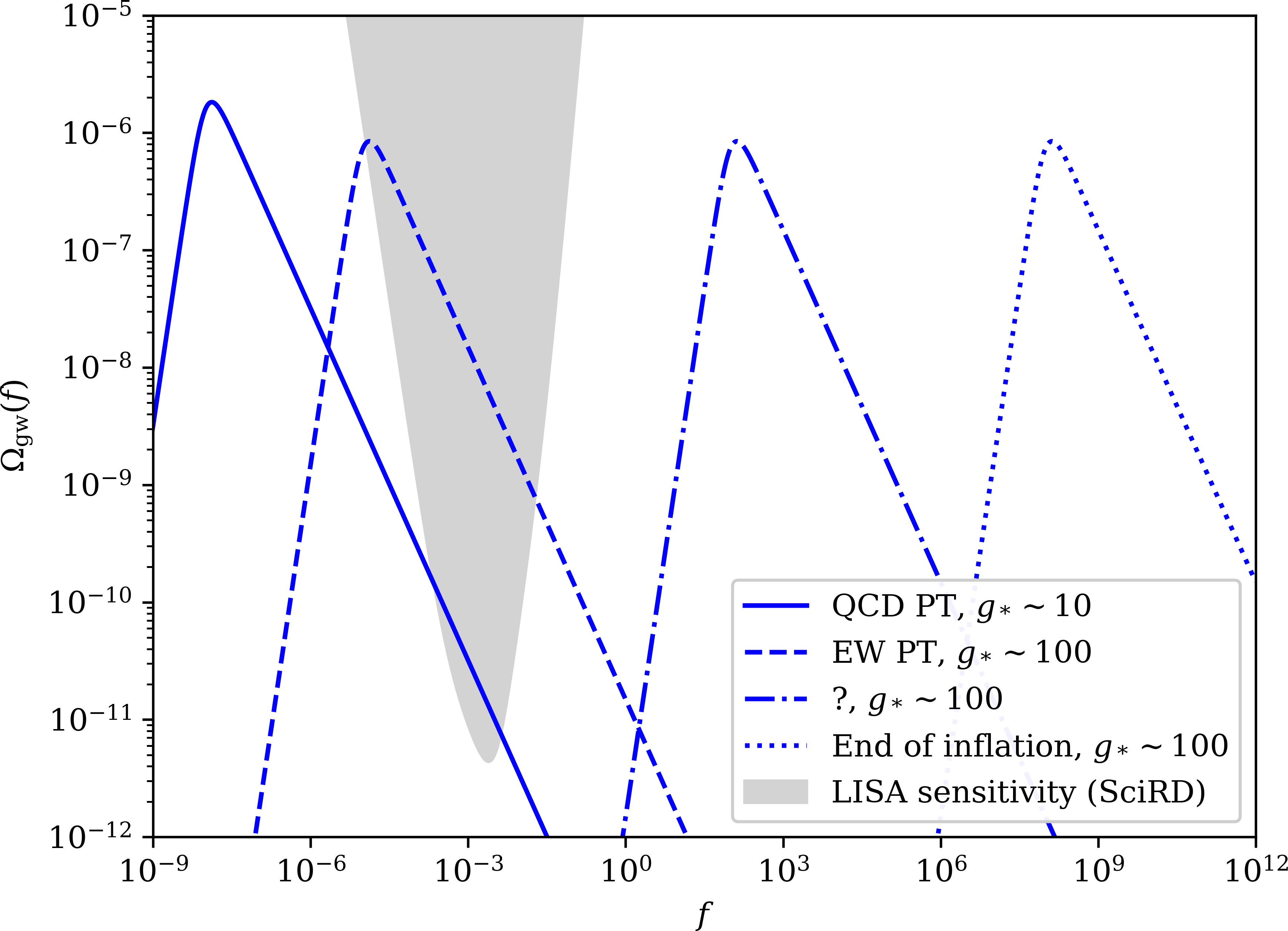
Typical frequencies
| Event | Time (s) | Temp (GeV) | $\mathbf{g}_*$ | Frequency (Hz) |
|---|---|---|---|---|
| QCD phase transition | $10^{-3}$ | $0.1$ | $\sim 10$ | $10^{-8}$ NANOGrav? |
| EW phase transition | $10^{-11}$ | $100$ | $\sim 100$ | $10^{-5}$ LISA! |
| ??? | $10^{-25}$ | $10^9$ | $\gtrsim 100$ | $100$ |
| End of inflation | $\gtrsim 10^{-36}$ | $\lesssim 10^{16}$ | $\gtrsim 100$ | $\gtrsim 10^8$ |
How $\rho_\text{gw}$ dilutes
- Gravitational waves behave like radiation, so their fraction of the energy in the universe does too: $$ \rho_{gw, 0} = \rho_\text{gw} \left( \frac{a(t_*)}{a(t_0)} \right)^4 $$
- ... and we know how to compute $\frac{a(t_*)}{a(t_0)}$, so $$ \begin{align} \rho_{gw, 0} & = \rho_\text{gw} \left( \frac{g_{*,s}(T_0)}{g_{*,s}(T_*)} \right)^{\frac{4}{3}} \left(\frac{T_0}{T_*}\right)^4 \\ & = \rho_\text{gw} \left( \frac{g_{*,s}(T_0)}{g_{*,s}(T_*)} \right)^{\frac{4}{3}} \frac{\rho_\text{rad,0}}{\rho_\text{rad}} \frac{g_*(T_*)}{g_*(T_0)}. \end{align} $$ using $\rho(T) = \frac{\pi^2}{30} g_*(T) T^4$ at the end.
Computing GW parameter $\Omega_\text{gw}$
- We have $$ \rho_{gw, 0} = \rho_\text{gw} \left( \frac{g_{*,s}(T_0)}{g_{*,s}(T_*)} \right)^{\frac{4}{3}} \frac{\rho_\text{rad,0}}{\rho_\text{rad}} \frac{g_*(T_*)}{g_*(T_0)}.$$
- We now dress things up to look more cosmological:
- Divide both sides by the present-day critical density $\rho_\text{c} \equiv 3 H_0^2/8\pi G$.
- Write things in terms of density parameters: $\Omega_\text{gw} \equiv \rho_\text{gw}/\rho_\text{c}$ for gravitational waves, and $\Omega_\text{rad} \equiv \rho_\text{rad}/\rho_\text{c}$ for radiation.
Parametrising our ignorance
- The critical density $\rho_\text{c} \equiv 3 H_0^2/8\pi G$ depends on the present day Hubble constant $H_0$.
- We would rather not depend on $H_0$, so multiply both sides by the reduced Hubble constant $h$, where $H_0 = h \times 100 \, \mathrm{km} \, \mathrm{s}^{-1} \,\mathrm{Mpc}^{-1}$.
- Planck and other big experiments/missions report cosmological parameters scaled by $h^2$ anyway.
- The formula then becomes $$ h^2 \Omega_\text{gw,0} = h^2 \Omega_\text{rad,0} \left( \frac{g_{*,s}(T_0)}{g_{*,s}(T_*)} \right)^{\frac{4}{3}} \frac{g_*(T_*)}{g_*(T_0)} \frac{\rho_\text{gw}}{\rho_\text{rad}}. $$
Filling in the numbers
- We can plug numbers into $$
h^2 \Omega_\text{gw,0} = h^2 \Omega_\text{rad,0} \left( \frac{g_{*,s}(T_0)}{g_{*,s}(T_*)}
\right)^{\frac{4}{3}}
\frac{g_*(T_*)}{g_*(T_0)} \frac{\rho_\text{gw}}{\rho_\text{rad}}.
$$
- $h^2 \Omega_\text{rad,0} \approx 4.18 \times 10^{-5}$ (CMB photons + neutrinos)
- $g_{*,s}(T_r) = 3.91$ and $g_{*}(T_r) = 3.36$
- Define $C = \rho_\text{gw}/\rho_\text{rad}$, fraction of (radiation-era) primordial energy turned into GWs, $C \ll 1$.
- With these quantities, we have $$ h^2 \Omega_\text{gw,0} = 4.18 \times 10^{-5} \left( \frac{3.91}{g_{*,s}(T_*)} \right)^{\frac{4}{3}} \frac{g_*(T_*)}{3.36} C.$$
Making $\Omega_\text{gw,0}$ cosmologist-friendly
- We cast $$ h^2 \Omega_\text{gw,0} = 4.18 \times 10^{-5} \left( \frac{3.91}{g_{*,s}(T_*)} \right)^{\frac{4}{3}} \frac{g_*(T_*)}{3.36} C.$$ again in 'familiar' terms by setting $g_{*,s}(T_*) \approx g_*(T_*)$ (okay for high temperatures).
- This yields $$ \begin{align} h^2 \Omega_\text{GW,0} & \approx 4.18\times 10^{-5} \times \frac{3.91^{\frac{4}{3}}}{3.36} \times 100^{-\frac{1}{3}} \left( \frac{100}{g_{*}(T_*)} \right)^{\frac{1}{3}} C \\ & \approx 1.65 \times 10^{-5} \left( \frac{100}{g_{*}(T_*)} \right)^{\frac{1}{3}} C. \end{align}$$
Power spectrum
- Consider an isotropic signal with spectral shape $$ \frac{1}{\rho_\text{rad}} \frac{\mathrm{d} \rho_\text{GW}(f)}{\mathrm{d} \ln f} = C S(f,f_*),$$ normalised such that $$ \frac{\rho_\text{GW}}{\rho_\text{rad}} = C \int \mathrm{d} f \frac{S(f,f_*)}{f}. $$
- Then we can directly apply the same formula to get $$ h^2 \frac{\mathrm{d} \Omega_\text{GW,0}(f)}{\mathrm{d}\ln f} \approx 1.65 \times 10^{-5} \left( \frac{100}{g_{*}(T_*)} \right)^{\frac{1}{3}} C S(f,f_*). $$
Power spectrum example
- If we take a traditionally popular example for primordial GWs: $$S(f,f_*) = N \frac{\left(f/f_*\right)^3}{1+\left(f/f_*\right)^4}.$$ then $N \approx 1.11$.
- And if we suppose $C \sim 0.1$, then $$ h^2 \frac{\mathrm{d} \Omega_\text{GW,0}(f)}{\mathrm{d}\ln f} \approx 1.49 \times 10^{-6} \left( \frac{100}{g_{*}(T_*)} \right)^{\frac{1}{3}} \frac{\left(f/f_*\right)^3}{1+\left(f/f_*\right)^4}. $$
(Very optimistic) examples
(Based on earlier table of numbers)
Day 4
- Thermodynamics of phase transitions
- How does LISA work?
- Production of GWs from phase transitions
Thermodynamics
Motivation
- In the previous section we described the various layers of approximation up to the field-fluid model.
- Now we will use that field-fluid model (and steady-state results) to explore the macroscopic behaviour of the wall.
- This is important both for baryogenesis and also for the GW power spectrum.
Further reading
- Energy budget: Espinosa, Konstandin, No and Servant arXiv:1004.4187
- More recent work: arXiv:2004.06995; arXiv:2010.09744.
Reaction front
- At a reaction front, there is a chemical transformation. The fluid is chemically and physically distinct on both sides.
- Different from a shock front, where the energy density and entropy change.
- We have a reaction front as $\langle \phi \rangle = 0$ before and $\langle \phi \rangle \neq 0$ after.
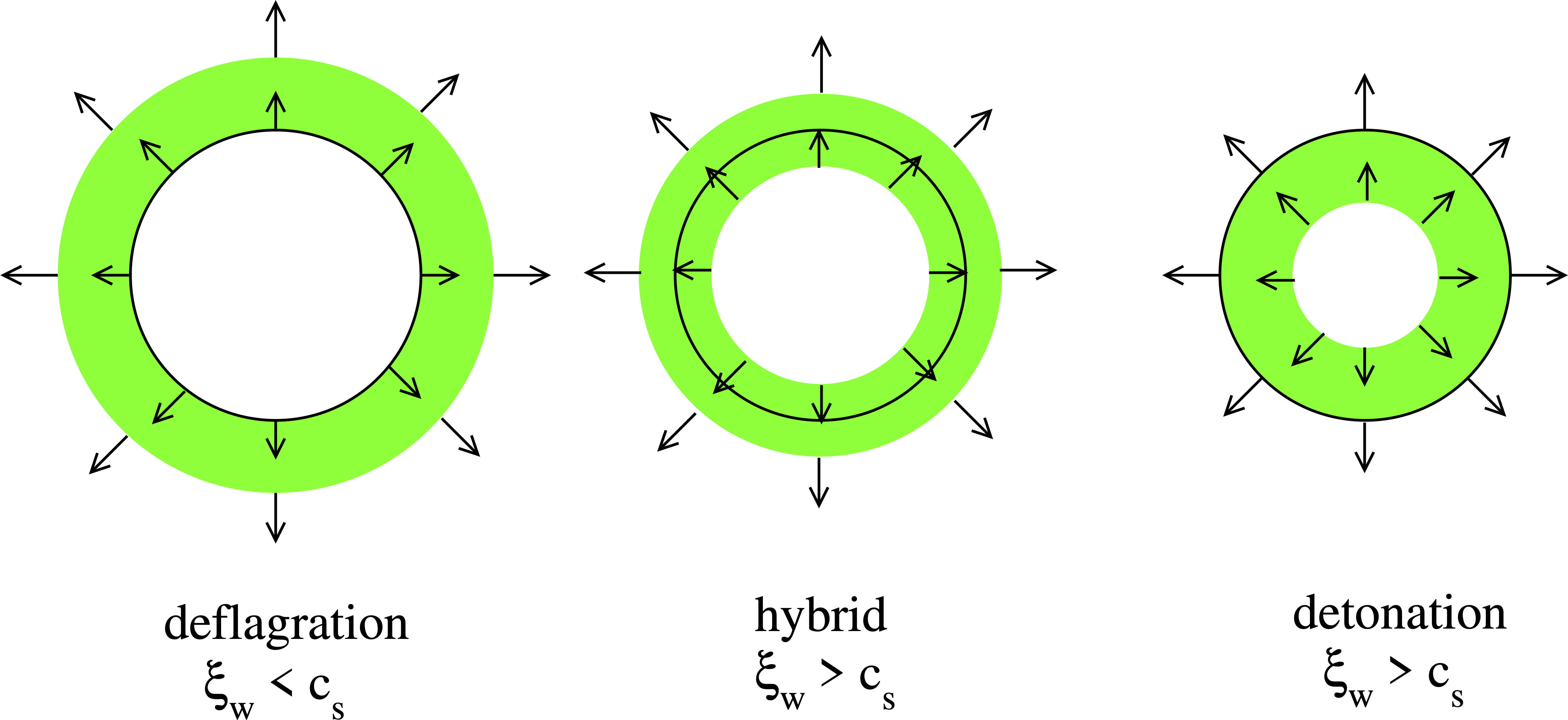
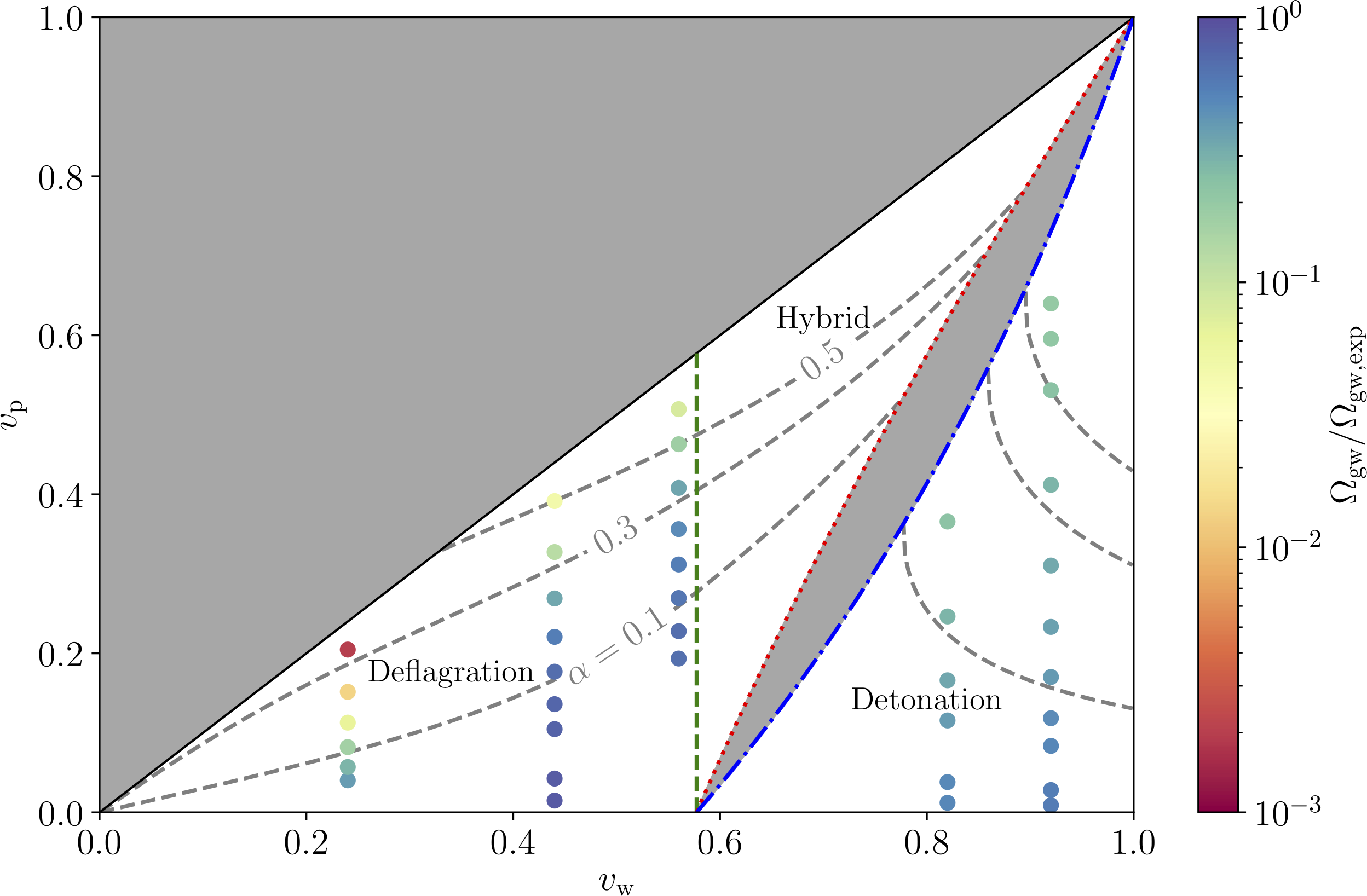
Detonations vs deflagrations
- If the scalar field wall moves supersonically and the fluid enters the wall at rest, we have a detonation
- If the scalar field wall moves subsonically and the fluid enters the wall at its maximum velocity, we have a deflagration
- Can also get a hybrid where the wall moves supersonically but some fluid bunches up in front of it, like a deflagration
Detonations, hybrids, deflagrations


Fluid profile equation
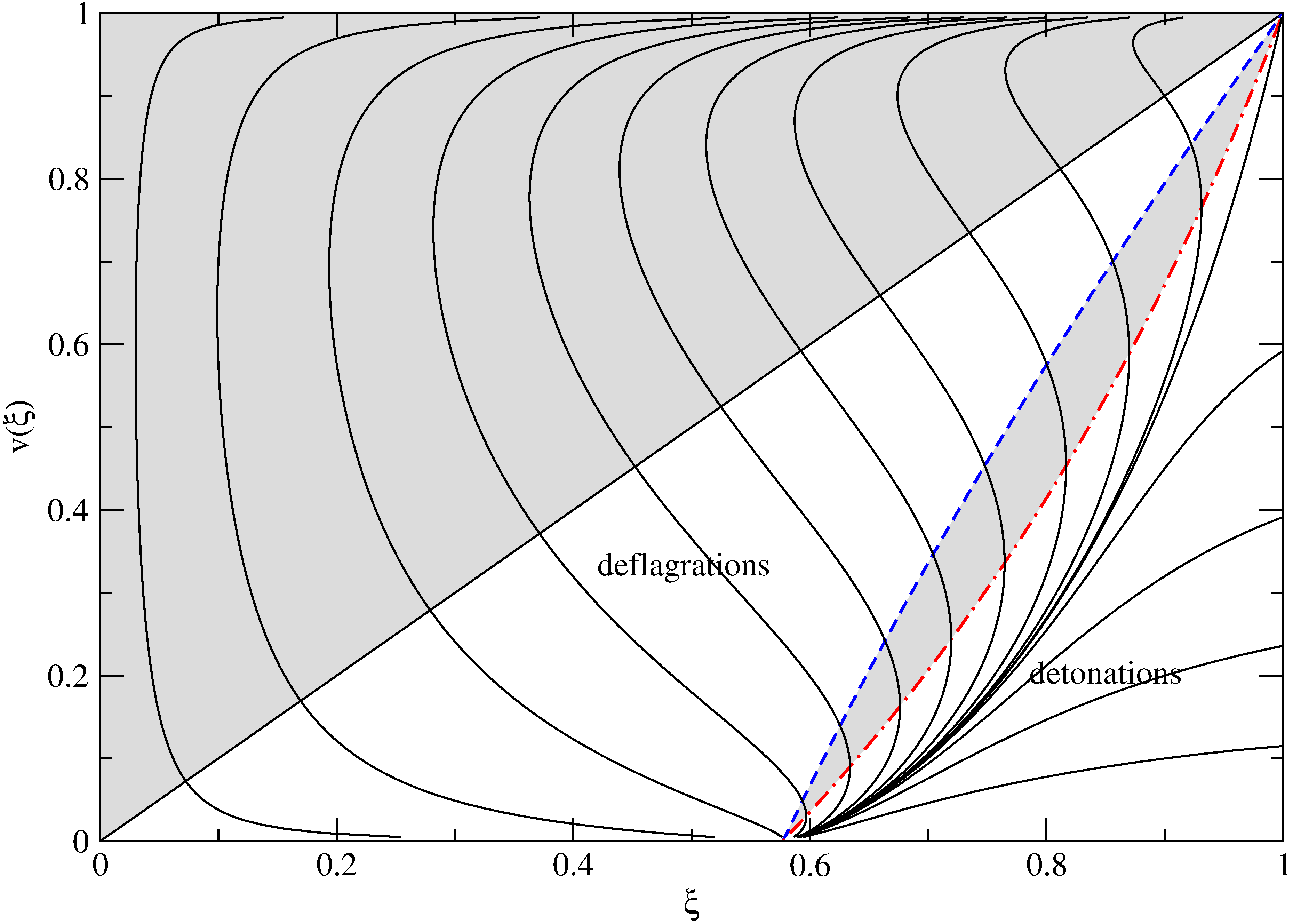
- As mentioned before, away from the bubble wall, there is no length scale in the fluid equations.
- Therefore expect that fluid profile around a spherical bubble will scale as $\text{radius}/\text{time}$: $\xi = r/t$
- Rearrange Euler equation to remove diffusion, using $c_\mathrm{s} = \sqrt{(\mathrm{d}p/dT)(\mathrm{d}\epsilon/dT)}$
- Then, if we know the fluid velocity we can solve $$ 2 \frac{v}{\xi} = \gamma^2(1- v\xi)\left[\frac{\mu^2}{c_s^2} - 1 \right] \frac{\partial v}{\partial \xi} $$ with the Lorentz-boosted fluid velocity $ \mu(\xi, v) = (\xi - v)/(1 - \xi v). $
Solution space
Junction conditions
- Energy conservation across the wall, in the wall frame (in $z$-direction) implies $\partial_z T^{zz} = \partial_z T^{z0} = 0$.
- Integrating these across the wall (from $+$ to $-$) yields
(enthalpy $w$, 3-velocity $v$, relativistic $\gamma$ and pressure $p$) $$ w_+ v_+^2 \gamma_+^2 + p_+ = w_- v_v^2 \gamma_-^2 + p_-, \qquad w_+ v_+ \gamma_+^2 = w_- v_- \gamma_-^2 $$ - Add an equation of state, e.g. bag model equation of state (and the phase transition strength $\alpha$), and we can solve for $v_+$, which gives us a starting point on our solution curves.
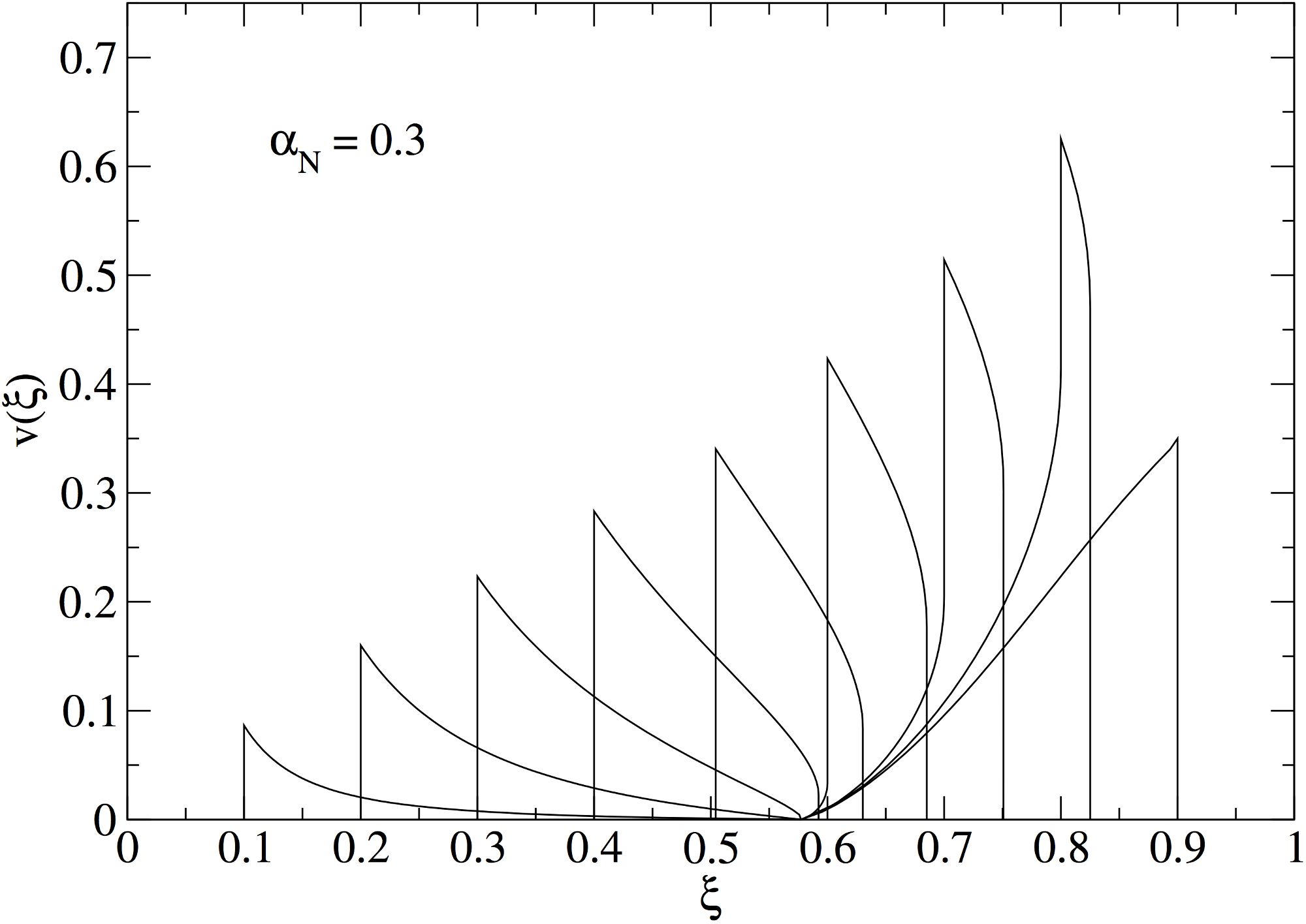
Fluid profiles
Phase transition strength
- The story so far:
- Bubbles nucleate (parameter $\beta$)
- Bubbles expand with finite velocity ($v_\mathrm{w}$)
- Fluid shell forms around bubble
- Latent heat $L$ ($+$ extra free energy difference) heats plasma...?
- Object of this section is to quantify how much of the latent heat ends up as kinetic energy.
One definition of $\alpha$
- Define phase transition strength $$ \alpha_L = \frac{L(T)}{g(T) \pi^2 T^4/30} = \frac{\text{latent heat at $T$}}{\text{radiation energy at $T$}} $$ which tell us how much of the energy of the universe was stored as latent heat in the phase transition.
- NB: there are multiple definitions of $\alpha$ in the literature, differing by what quantifies the 'available energy' (latent heat, trace anomaly, vacuum energy)
- Larger $\alpha_T$ ⇒ stronger phase transition
Another, better definition of $\alpha$
- Define the trace anomaly $\theta(T) = \frac{1}{4} (\epsilon(T) - 3p (T))$, where $\epsilon$ and $p$ are energy density and pressure of the plasma.
- (trace anomaly can be calculated on the lattice using the same methods as we discussed yesterday)
- Then $\alpha_\theta$ is defined as ('ms' = 'metastable') $$ \alpha_\theta = \frac{1}{\epsilon_Q(T)}\left(\theta_\text{ms}(T) - \theta_\text{stable}(T)\right); \quad \epsilon_Q(T) = \frac{3}{4}(\underbrace{\epsilon(T) + p (T)}_\text{enthalpy, $w$})$$
- Agrees with $\alpha_L$ at small supercooling.
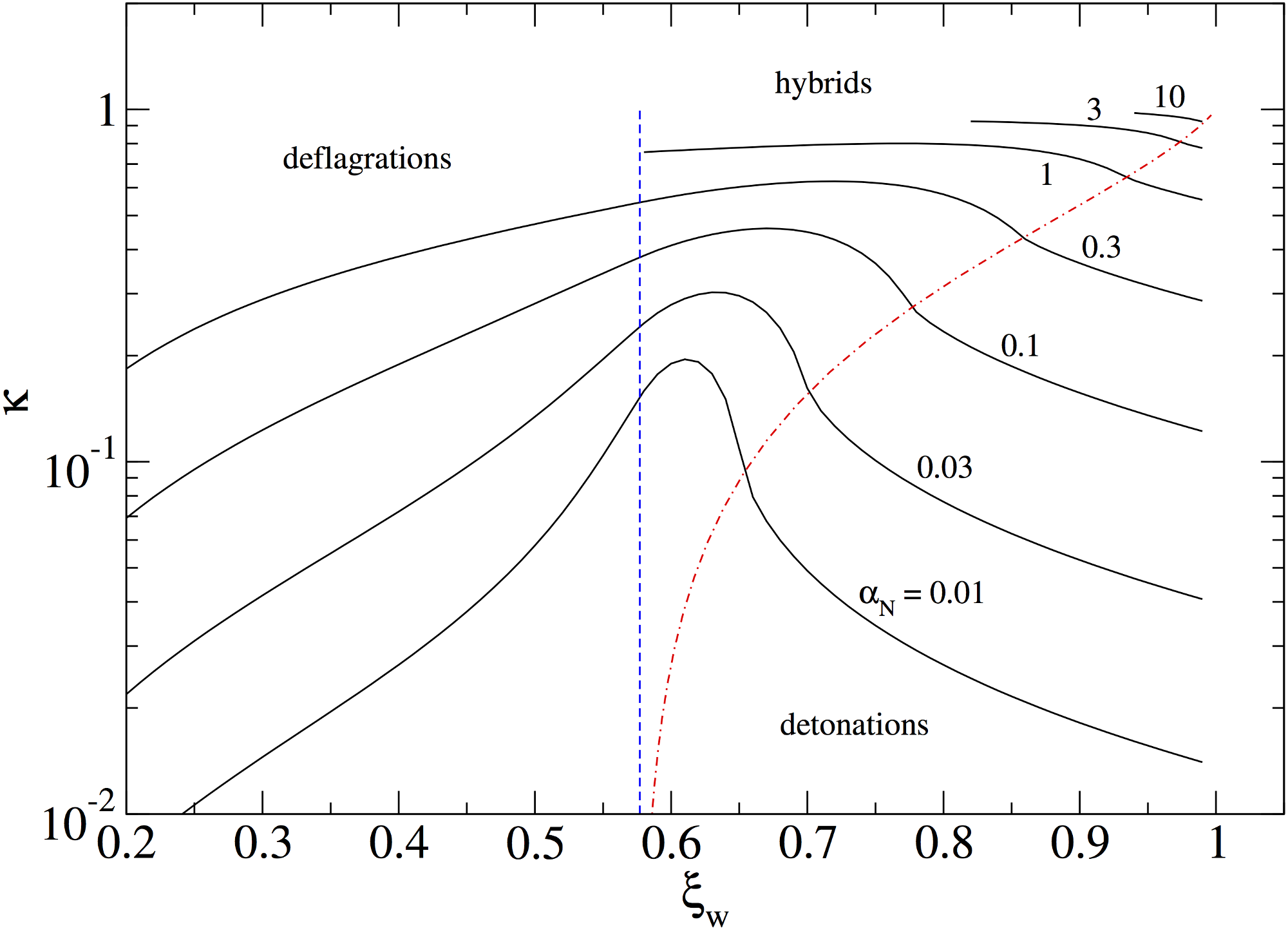
Computing the efficiency
- But $\alpha_T$ does not say how much of $\mathcal{L}$ ends up as fluid kinetic energy
- For that we define the efficiency $$ \kappa_\mathrm{f} = \frac{\overbrace{(\epsilon + p) u_i u_i}^{T^{00}_\text{fluid}}}{L}= \frac{\text{fluid KE}}{\text{latent heat}}$$
- Then $\kappa_\mathrm{f} \alpha_T$ is the fraction of the energy density in the universe that ends up as fluid kinetic energy.
- Very roughly, $\kappa_\mathrm{f} \alpha_T \approx \overline{U}_f^2$, the (weighted) mean square fluid velocity as the transition completes.
- Can be computed more accurately either from spherical simulations or directly solving.
Efficiency curves
Thermodynamics: conclusion
- Thermal first-order transitions have a reaction front
- Reaction fronts can be deflagrations (generally subsonic), detonations (supersonic) or hybrids (a mixture).
- The fluid reaches a scaling profile in $\xi = r/t$ based on the available latent heat and wall velocity.
- From this, one can compute the efficiency $\kappa_\mathrm{f}$ and hence how much of the energy in the universe ends up in the fluid $\kappa_\mathrm{f} \alpha_T$.
Summary
- What parameters have we introduced?
- Equilibrium lattice simulations: $T_c$ (and $\sigma$, $L$)
- Nucleation: inverse duration $\beta$ (and hence $T_n$)
- Wall velocities: $v_\mathrm{w}$
- Thermodynamics: $\alpha$ and $\kapps$
- That is everything we need to know about the physics of the phase transition, so we can now talk about the production of GWs.
LISA and how it works
LISA is coming!
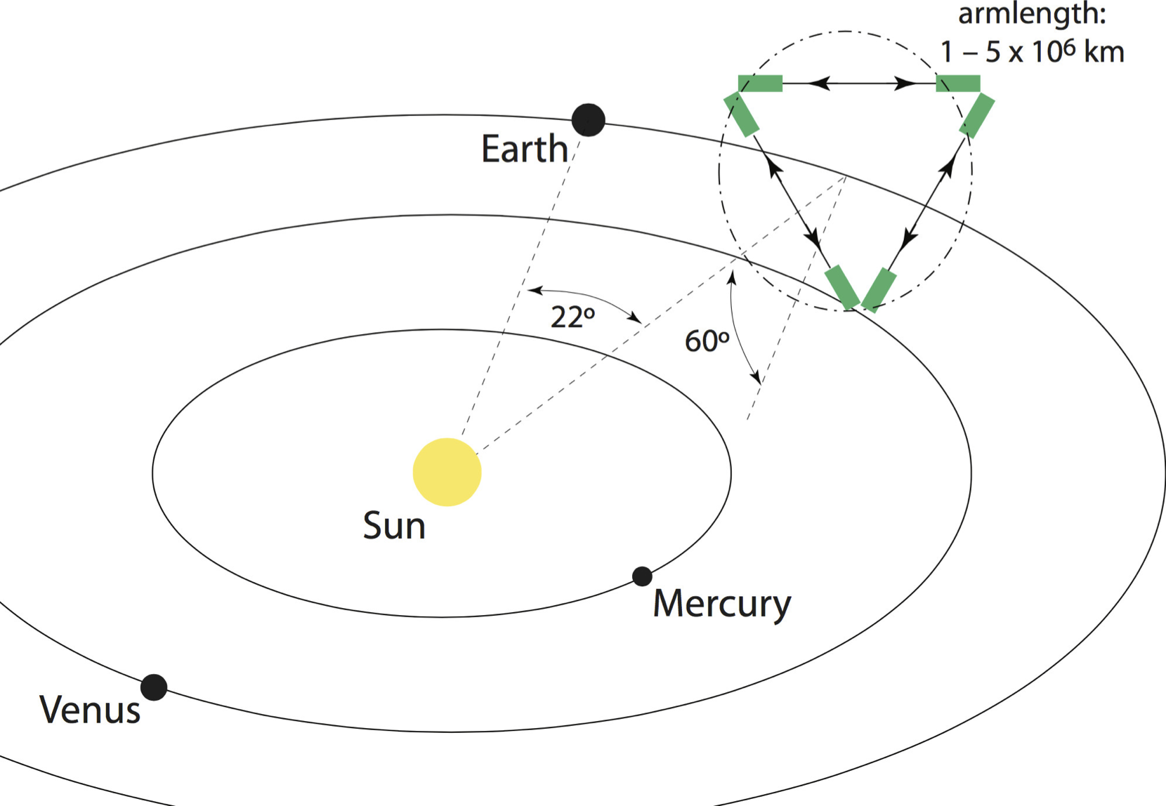
- Three laser arms, 2.5 M km separation
- ESA-NASA mission, launch 2030s
- Mission exited 'phase A' in December 2021
Source: [PD] NASA via Wikimedia Commons
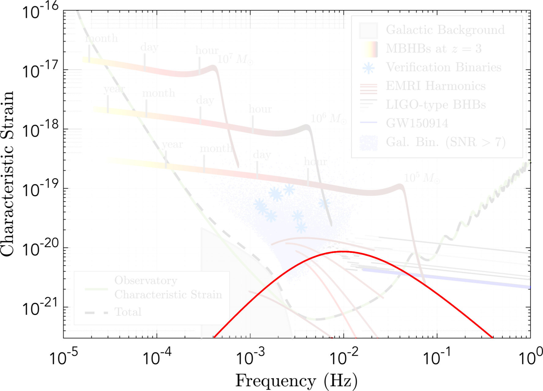
LISA: "Astrophysics" signals
Source: arXiv:1702.00786
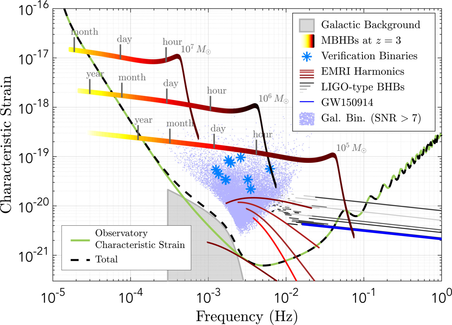
LISA: Stochastic background?
[qualitative curve, sketched on]
From the proposal
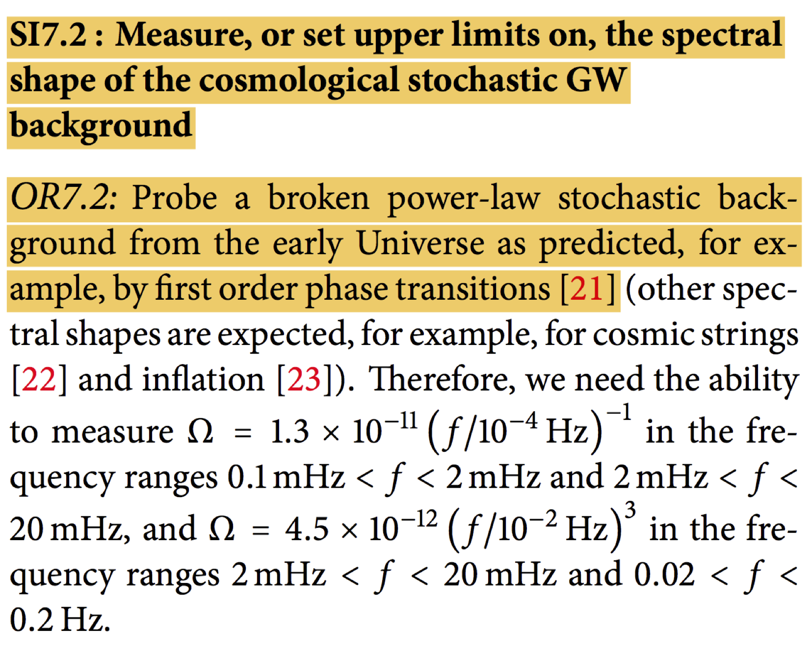
Source: LISA proposal.
Where does the sensitivity curve come from?
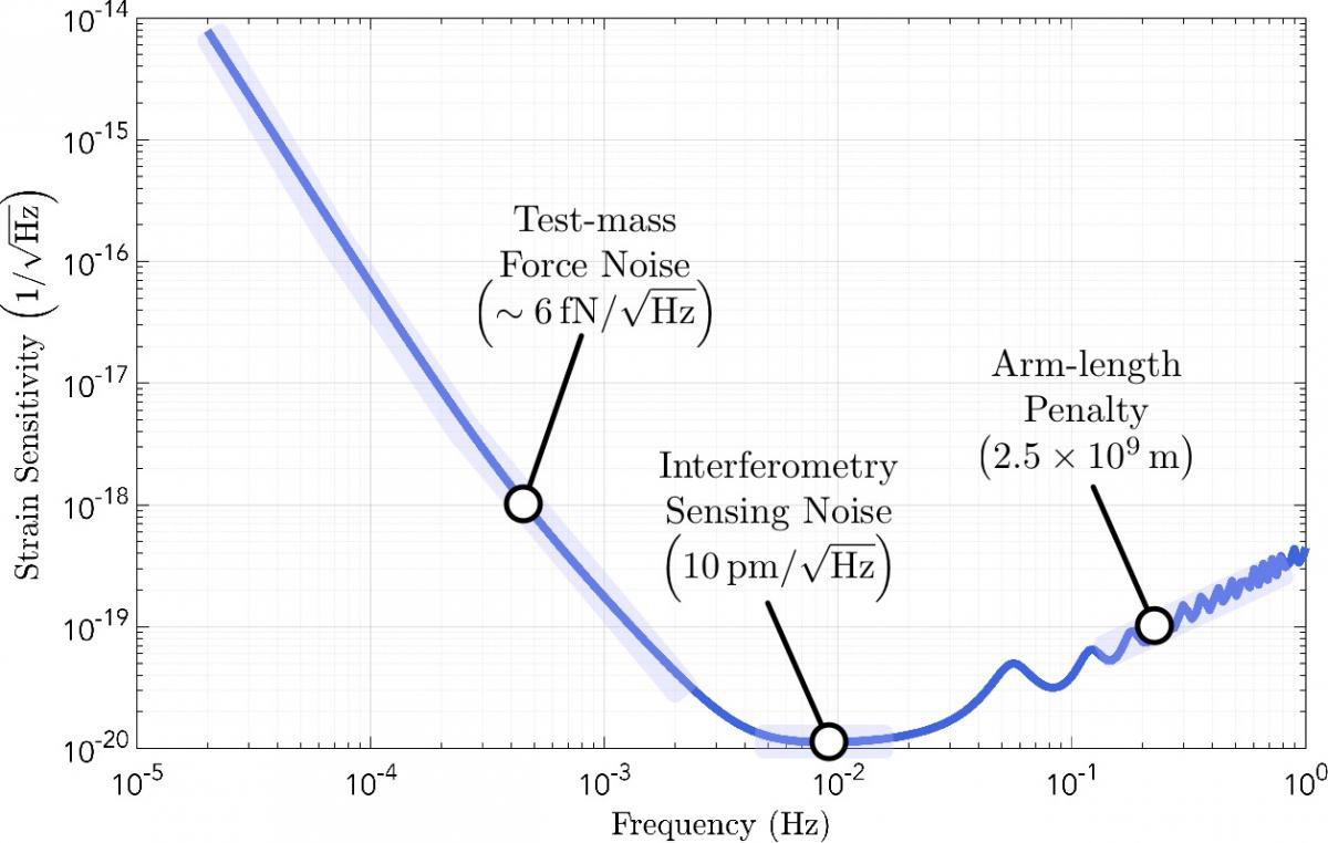
From lisamission.org L3 mission proposal
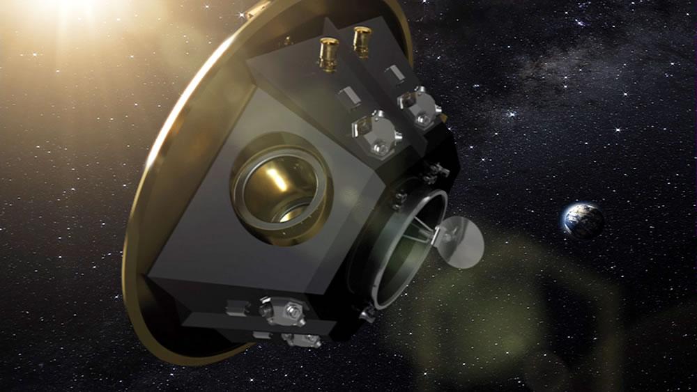
What does LISA look like?
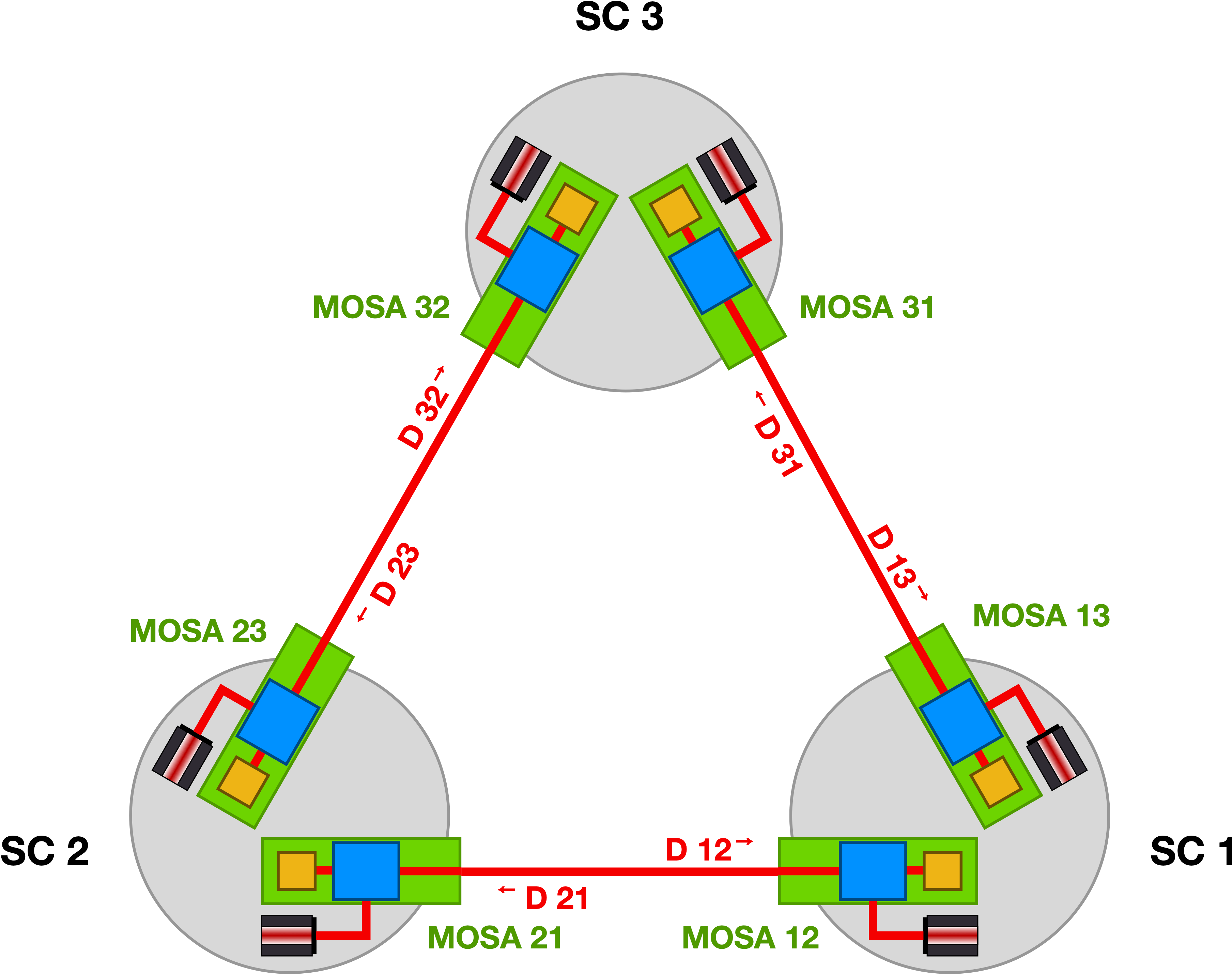
SC = spacecraft; MOSA = movable optical sub assembly
Contains optical bench (blue) and test mass (yellow)
From arXiv:2103.06976
How does LISA work?
- Spacecraft $j$ sends a laser with phase $\Phi_j$ to spacecraft $i$, which is received at time $t$: $$ \Phi_{i \leftarrow j} = \Phi_j(t - d_{ij}(t) - H_{ij}(t)) $$ where $d_{ij}$ is the light travel time, and $H_{ij}$ is an additional delay due to GWs
- Taylor expanding about $t - d_{ij}$ $$ \Phi_{i \leftarrow j} = \Phi_j(t - d_{ij}) - \dot{\Phi}_j (t - d_{ij})H_{ij}(t),$$
- introducting a delay operator $\mathbf{D}_{ij} x(t) = x(t-d_{ij}(t))$: $$ \Phi_{i \leftarrow j} = \mathbf{D}_{ij}\Phi_j - (\mathbf{D}_{ij} \dot{\Phi}_j) H_{ij}$$
Beats and noises
- Denote $\dot{\Phi}_i = \nu_i$, a frequency, and so the frequency of the received beam is $$ \begin{align}\nu_{i \leftarrow j} \equiv \dot{\Phi}_{i \leftarrow j} & = \left[1-\dot{d}_{ij}(t)- \dot{H}_{ij}(t)\right] \\ & \qquad \times \left[\nu_j(t-d_{ij}(t) - \dot{\nu}_j(t-d_{ij}(t))H_{ij}(t))\right]\end{align}$$
- Neglecting terms $\dot{\nu}_j H_{ij}$, $$\nu_{i \leftarrow j} = (1-\dot{d}_{ij})\mathbf{D}_{ij}\nu_j - (\mathbf{D}_{ij}\nu_j)\dot{H}_{ij}$$
- On spacecraft $i$ this is compared with the local laser $\Phi_j(t)$, $\Phi^\text{isc}_{ij}(t) \equiv \Phi_{i\leftarrow j}(t) - \Phi_i(t)$, to get $$ \nu_{ij}^\text{isc} = (1-\dot{d}_{ij})\mathbf{D}_{ij}\nu_j - \nu_i - (\mathbf{D}_{ij}\nu_j)\dot{H}_{ij}$$
Beatnote frequency
- $\nu_{ij}^\text{isc}$ measures the frequency of the beats
- Cannot neglect laser noise (fluctuations in $\nu_i$ and $\nu_j$): it will always be bigger than the GW signal $(\mathbf{D}_{ij}\nu_j)\dot{H}_{ij}$.
- Time-domain interferometry (TDI): take advantage of the same laser noise appearing in different measurements to cancel it out.
- This uses quantities like (Michelson variables): $$ \begin{multline} X = \left(\mathbf{D}_{31}\mathbf{D}_{13}\mathbf{D}_{21} \nu_{12} + \mathbf{D}_{31}\mathbf{D}_{13}\nu_{21} + \mathbf{D}_{31}\nu_{13} + \nu_{31}\right) \\ - \left(\nu{21} + \mathbf{D}_{21}\nu{12} + \mathbf{D}_{21}\mathbf{D}_{12}\nu_{31} + \mathbf{D}_{21}\mathbf{D}_{12}\mathbf{D}_{31}\nu_{13}\right) \end{multline} $$ (and cyclic permutations $Y$, $Z$)
- Higher order combinations handle realistic scenarios.
TDI sketch
GWs from primordial physics
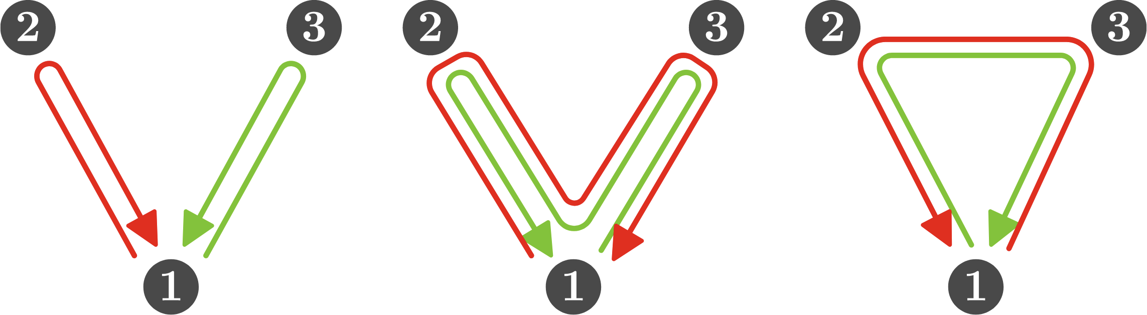
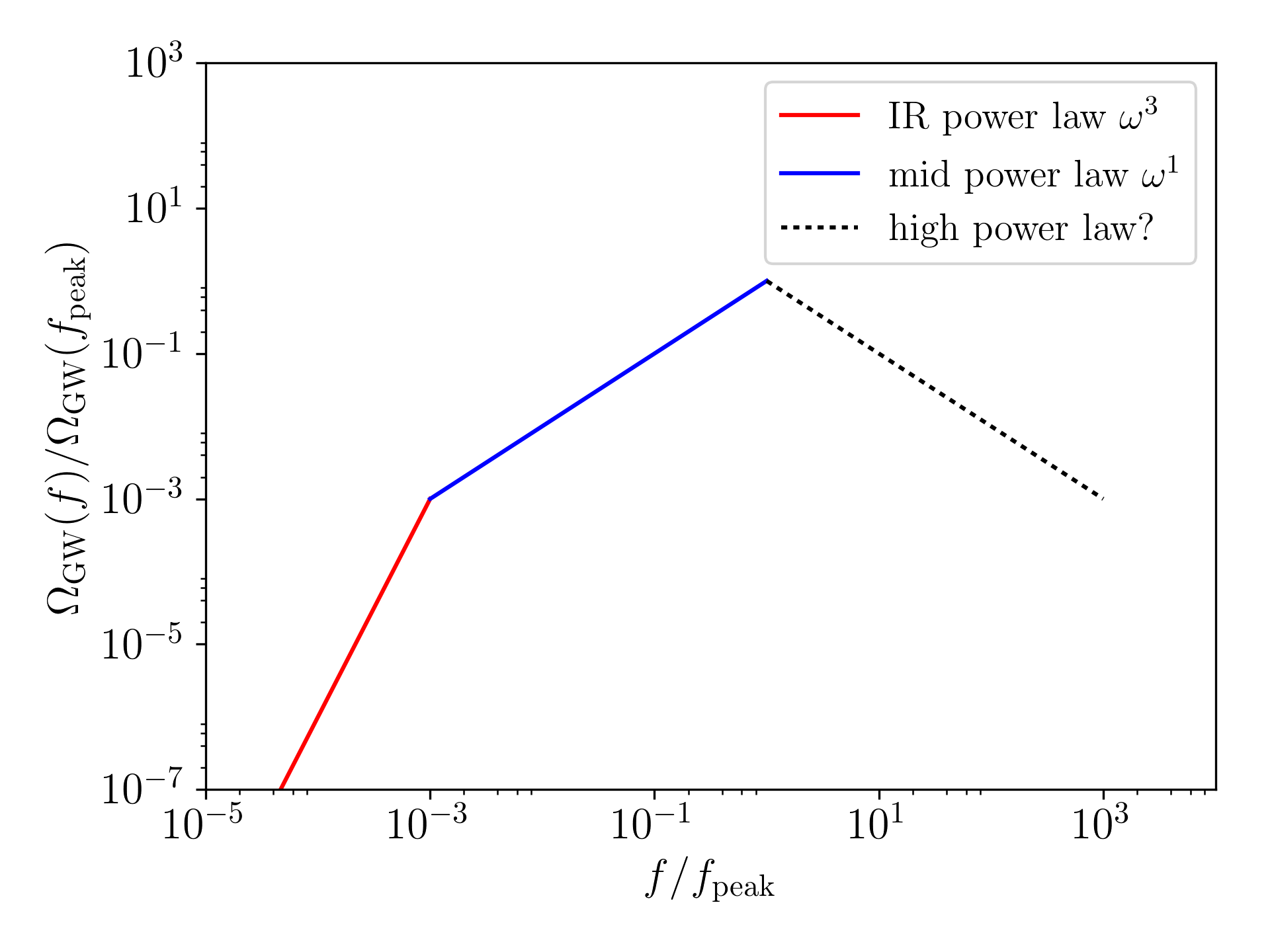
Useful insight 1
Source: Dufaux, Felder, Kofman, Navros
- Begin with the momentum-space Green's function expression (assume source off at $t' < 0$) $$ h_{ij}^\text{TT}(\mathbf{k},t)=16\pi G \, \Lambda_{ij,lm} \int_0^t \, \mathrm{d} t' \frac{\sin[k(t-t')]}{k} T_{lm}(\mathbf{k},t') $$
- If the source is slowly varying in space at low $\mathbf{k}$: $$T_{lm}(\mathbf{k}) \to \text{const.}; \qquad k \ll k_\text{max} $$ we get $$ h_{ij}^\text{TT}(\mathbf{k},t) \approx 16\pi G \, \Lambda_{ij,lm} \int_0^t \, \mathrm{d} t' \frac{\sin[k(t-t')]}{k} T_{lm}(0,t') $$
Useful insight 1
- If the source $T_{lm}(0,t)$ varies faster than the $\sin[k(t-t')]$, the equation reduces to $$ h_{ij}^\text{TT}(\mathbf{k},t) \approx 16\pi G \, \Lambda_{ij,lm} \int_0^t \, \mathrm{d} t' T_{lm}(0,t') $$ This gives $$ \frac{\mathrm{d} \rho_\text{GW}(k)}{\mathrm{d} \, \log \, k} \propto k^3 $$
- In other words, at sufficiently long sub-horizon scales, all that matters is how long the source is on for.
- The power law is $k^3$.
- This holds for any subhorizon physics.
Useful insight 2
- If the source has an intermediate regime where $T_{lm}(0,t)$ varies slower than $\sin[k(t-t')]$, then the source stays in the integral, and there is an additional $1/k$ factor
- Therefore, in some cases we can expect a $k^1$ power law at higher wavenumbers than the $k^3$ is valid
Useful insight: graphical summary
Simulating first order phase transitions: simulations
Recap: what happens?
- Bubbles nucleate (temperature $T_\mathrm{N}$, on timescale $\beta^{-1}$)
- Bubble walls expand in a plasma (at velocity $v_\mathrm{w}$)
- Reaction fronts form around walls (with strength $\alpha$)
- Bubbles + fronts collide GWs
- Sound waves left behind in plasma GWs
- Shocks [$\rightarrow$ turbulence] $\rightarrow$ damping GWs
Reminder: coupled field-fluid system
Ignatius, Kajantie, Kurki-Suonio and Laine- Simulate Scalar $\phi$ and ideal fluid $u^\mu$.
- Split stress-energy tensor $T^{\mu\nu}$ into field and fluid bits $$\partial_\mu T^{\mu\nu} = \partial_\mu (T^{\mu\nu}_\text{field} + T^{\mu\nu}_\text{fluid}) = 0$$
- Parameter $\eta$ sets the scale of friction due to plasma $$\partial_\mu T^{\mu\nu}_\text{field} = \tilde \eta \frac{\phi^2}{T} u^\mu \partial_\mu \phi \partial^\nu \phi \quad \partial_\mu T^{\mu\nu}_\text{fluid} = - \tilde \eta \frac{\phi^2}{T} u^\mu \partial_\mu \phi \partial^\nu \phi $$
- $V(\phi,T)$ is a 'toy' effective potential
- $\beta$ ↔ number of bubbles; $\alpha_{T_*}$ ↔ $\Delta V(\phi, T_*)$, $v_\text{wall}$ ↔ $\tilde \eta$
Dynamic range issues
- Most realtime lattice simulations in the early universe have a single [nontrivial] length scale
- Here, many length scales important
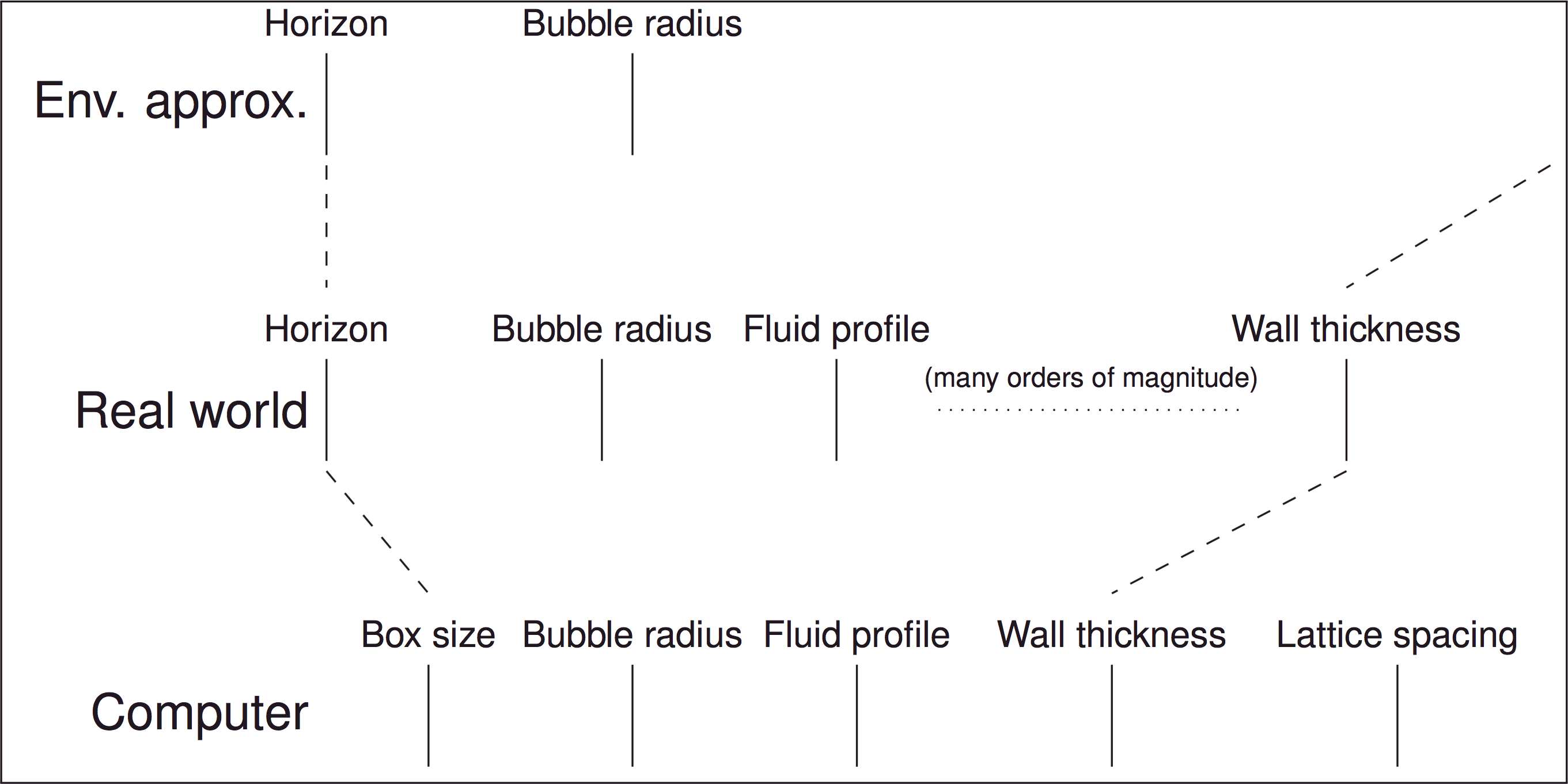
Eulerian implementation
Different things live in different places...
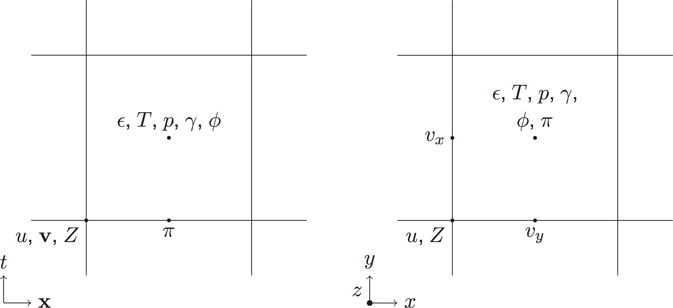
Summary of algorithm 1:
- Original eom is: $$ (\partial_\mu \partial^\mu \phi) - \frac{\partial V_\text{eff}(\phi,T)}{\partial \phi} = -\eta(\phi, v_\mathrm{w}) u^\mu \partial_\mu \phi $$
- Use leapfrog + Crank-Nicolson algorithms: $$\begin{align} \phi(x, t+\delta t) & = \phi(x,t) + \delta t \, \pi(x,t + \delta t/2) \\ \pi(x, t+\delta t/2) & = \frac{1}{1-z}\Bigg[(1+z)\pi(x, t-\delta t/2) + \delta t \bigg( \nabla^2 \phi(x, t) \\ & \qquad - \frac{\partial V_\text{eff}(\phi,T)}{\partial \phi} + \eta(\phi, v_\mathrm{w}) u^i \partial_i \phi(x,t) \bigg)\Bigg] \\ \end{align} $$ where $z = - \delta t \, \eta(\phi, v_\mathrm{w}) \gamma $.
Summary of algorithm 2:
- Metric perturbations also evolved with leapfrog.
- Equation of motion is $$ - \ddot{h}_{ij}(x,t) +\nabla^2 h_{ij}(x,t) = 16 \pi G T^\text{source}_{ij}(x,t). $$ where the sources are $$ T^{\text{source},\,\phi}_{ij} = \partial_i \phi \partial_j \phi; \qquad T^{\text{source},\,\text{fluid}} = w u_i u _j $$
- This becomes $$ \begin{align} h_{ij}(x, t+\delta t) & = h_{ij}(x,t) + \delta t \, \dot{h}_{ij}(x,t+\delta t /2) \\ \dot h_{ij}(x, t+\delta t/2) & = \dot h_{ij}(x, t-\delta t/2) + \delta t\, \big[ \nabla^2 h_{ij}(x, t) \\ & \qquad + 16 \pi G T^\text{source}_{ij} (x, t) \big] \end{align}$$
Summary of algorithm 3:
- The fluid eom was $$ \partial_\mu (w u^\mu u^\nu) - \partial^\nu p + \frac{\partial V_\text{eff}(\phi,T)}{\partial \phi} \partial^\nu \phi = + \eta(\phi, v_\mathrm{w}) u^\mu \partial_\mu \phi \partial^\nu \phi $$
- Solving this accurately is rather more involved!
Operator splitting methods... Wilson and Matthews- Pressure acceleration
- Update velocities ($u_i$, $V_i$), gamma-factors
- Pressure work on fluid
- Advection of state variables
- Update velocities again
- Pressure work again
Velocity profile development: small $\tilde \eta$ ⇒ detonation (supersonic wall)
Velocity profile development: large $\tilde \eta$ ⇒ deflagration (subsonic wall)
Real time simulation example
Velocity power spectra
Fast deflagration
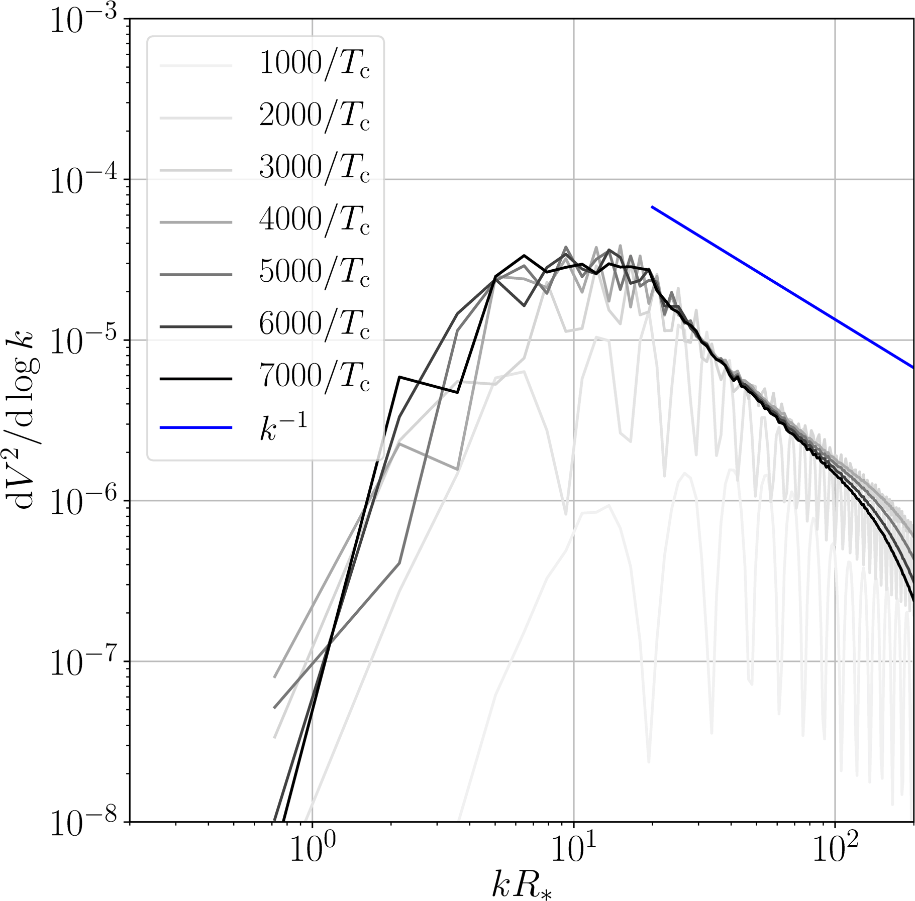
Detonation
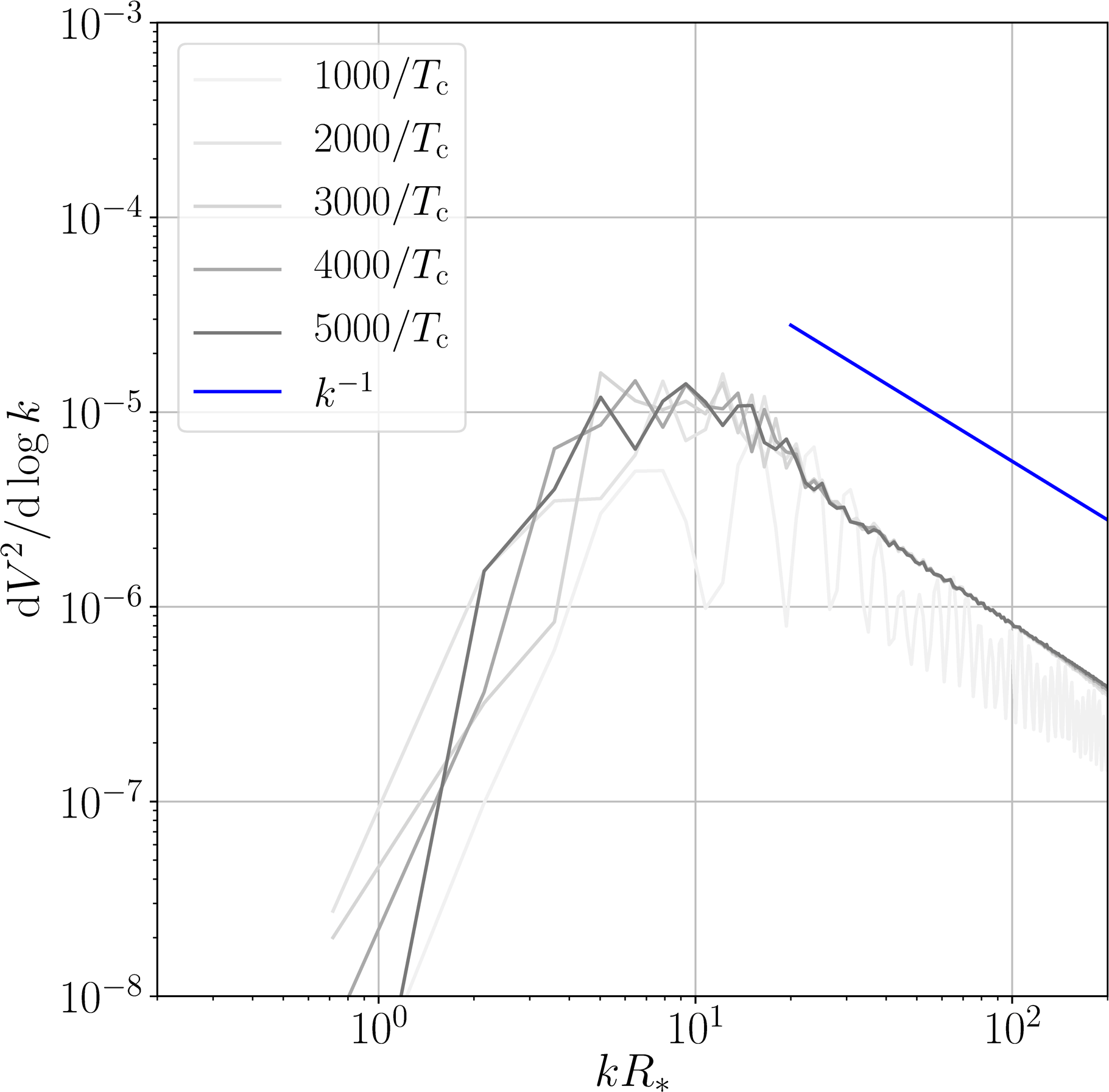
- Weak transition: $\alpha_{T_*} =0.01$
- Power law above peak is between $k^{-2}$ and $k^{-1}$
- (Spurious “ringing” due to simultaneous nucleation)
From $\phi$ and $u_\mu$ to $h_{ij}$ and $\Omega_\text{GW}$
- As discussed, simply evolve: $$ \square h_{ij}(x,t) = 16 \pi G T_{ij}^\text{source}(x,t). $$
- Note that when $T_{ij}^\text{source}(x,t) =
w(x)u_i(x)u_j(x)$ this is basically a convolution of the
fluid velocity power
(assuming $w(x) \approx \bar w$) Caprini, Durrer and Servant - When we want to measure the energy in gravitational waves, we do the projection to TT and measure: $$ t_{\mu\nu}^\text{GW}= \frac{1}{32 \pi G}\langle \partial_\mu h^\text{TT}_{ij} \partial_\nu h^\text{TT}_{ij} \rangle; \quad \rho_\text{GW} = \frac{1}{32 \pi G} \langle \dot{h}^\text{TT}_{ij} \dot{h}^\text{TT}_{ij} \rangle. $$
- We can then redshift this to present day to get $\Omega_\text{GW} h^2$.
GW power spectra and power laws
Fast deflagration
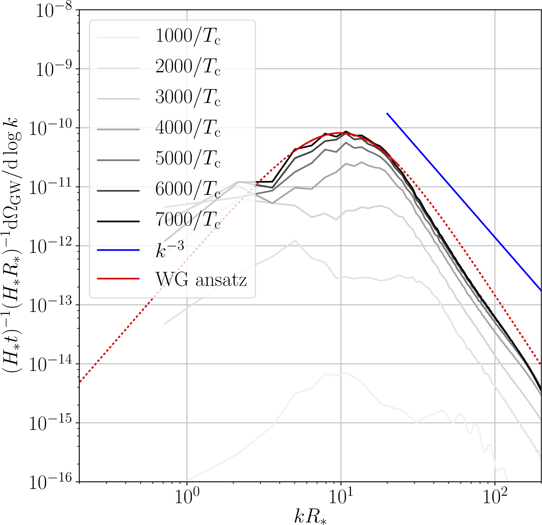
Detonation
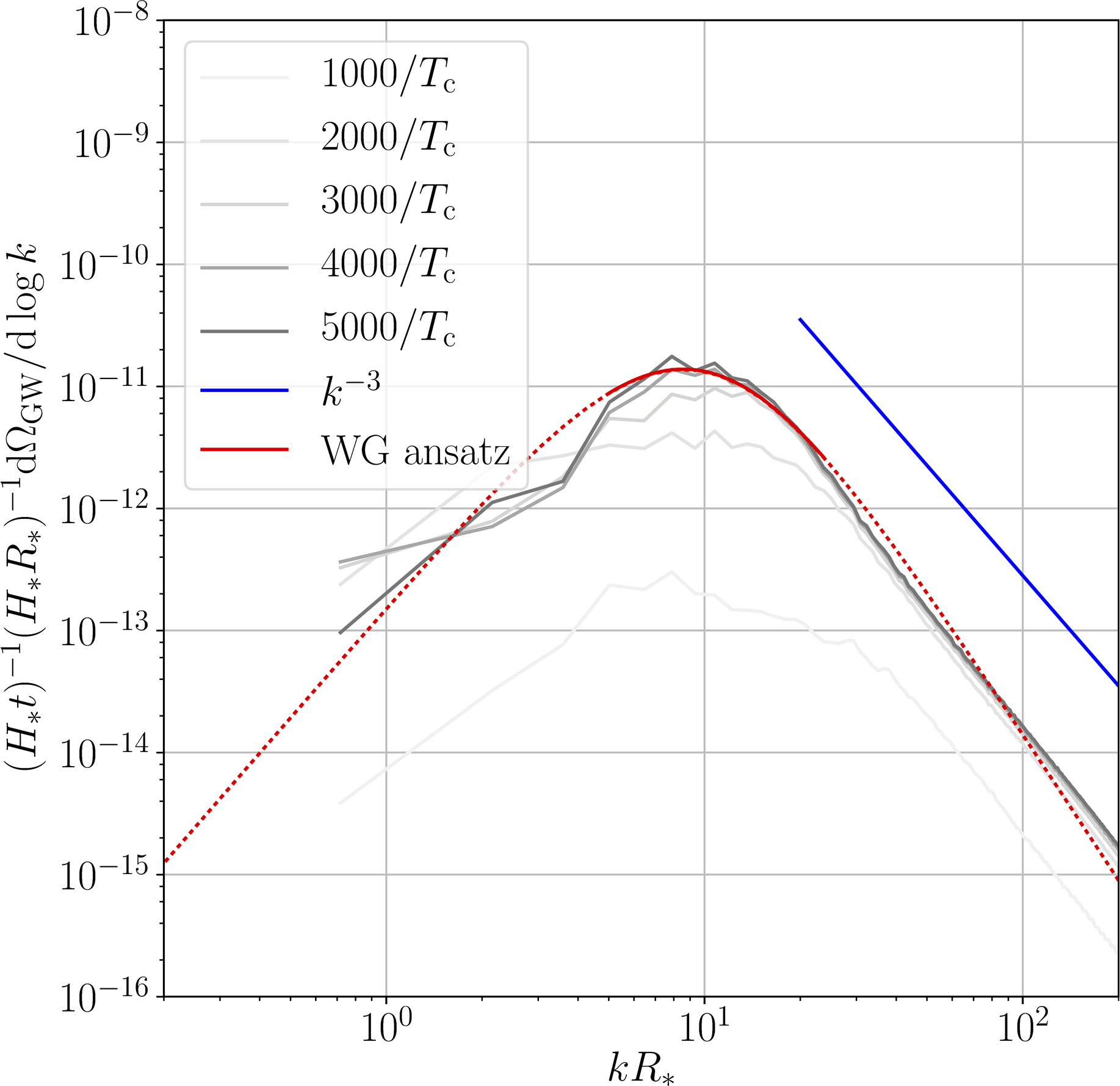
- Causal $k^3$ at low $k$, approximate $k^{-3}$ or $k^{-4}$ at high $k$
- Curves scaled by $t$: source until turbulence/expansion
Simulations: conclusion
- Need to compress a lot of length scales into our box.
- Current cutting-edge simulations are still frustratingly small in size, need to extrapolate.
- Therefore, use simulation results to derive ansätze
and models, and combine with theoretical results where
required to make predictions
example: Sound Shell Model arXiv:1608.04735
GWs from first order phase transitions: recent results
Nonlinearities?
- Nonlinearities during the transition:
- Generation of vorticity
- Formation of droplets
- Nonlinearities after the transition:
- Fluid motion becomes nonlinear on a time scale
$$\tau_\text{sh} = \frac{R_*}{\overline{U}} = \frac{\text{Bubble radius (i.e. typical length scale)}}{\text{Typical fluid velocity}}$$ - Then come shocks and turbulence
(Kolmogorovand acoustic)
- Fluid motion becomes nonlinear on a time scale
Strong deflagrations ⇒ droplets
[$\alpha_{T_*} = 0.34$, $v_\mathrm{w} = 0.24$ (deflag.)], velocity $\mathbf{v}$
A closer look in spherical geometry
Droplets form ➤ walls slow down
At large $\alpha_{T_*}$ reheated droplets form in front of the walls
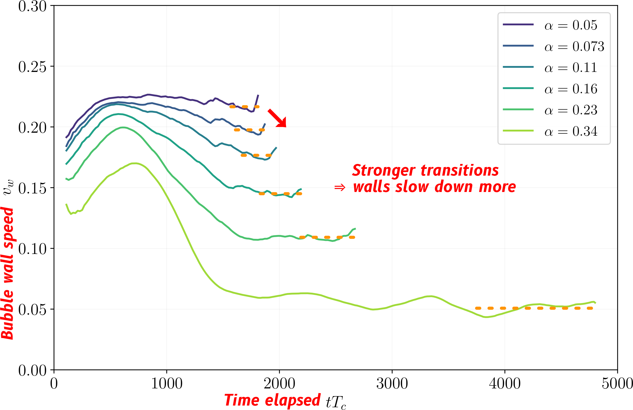
Droplets may suppress GWs
case
scenario ➘
Droplets and phenomenology
- Long-lived regions with moderate wall velocities
- Could this help with baryogenesis? For strong transitions, walls often move too quickly.
- Proposals for dark strongly interacting matter 'nuggets' where the phases coexist e.g. arXiv:1810.04360 arXiv:1912.02830
- Other applications?
- Further 3D simulations will be needed
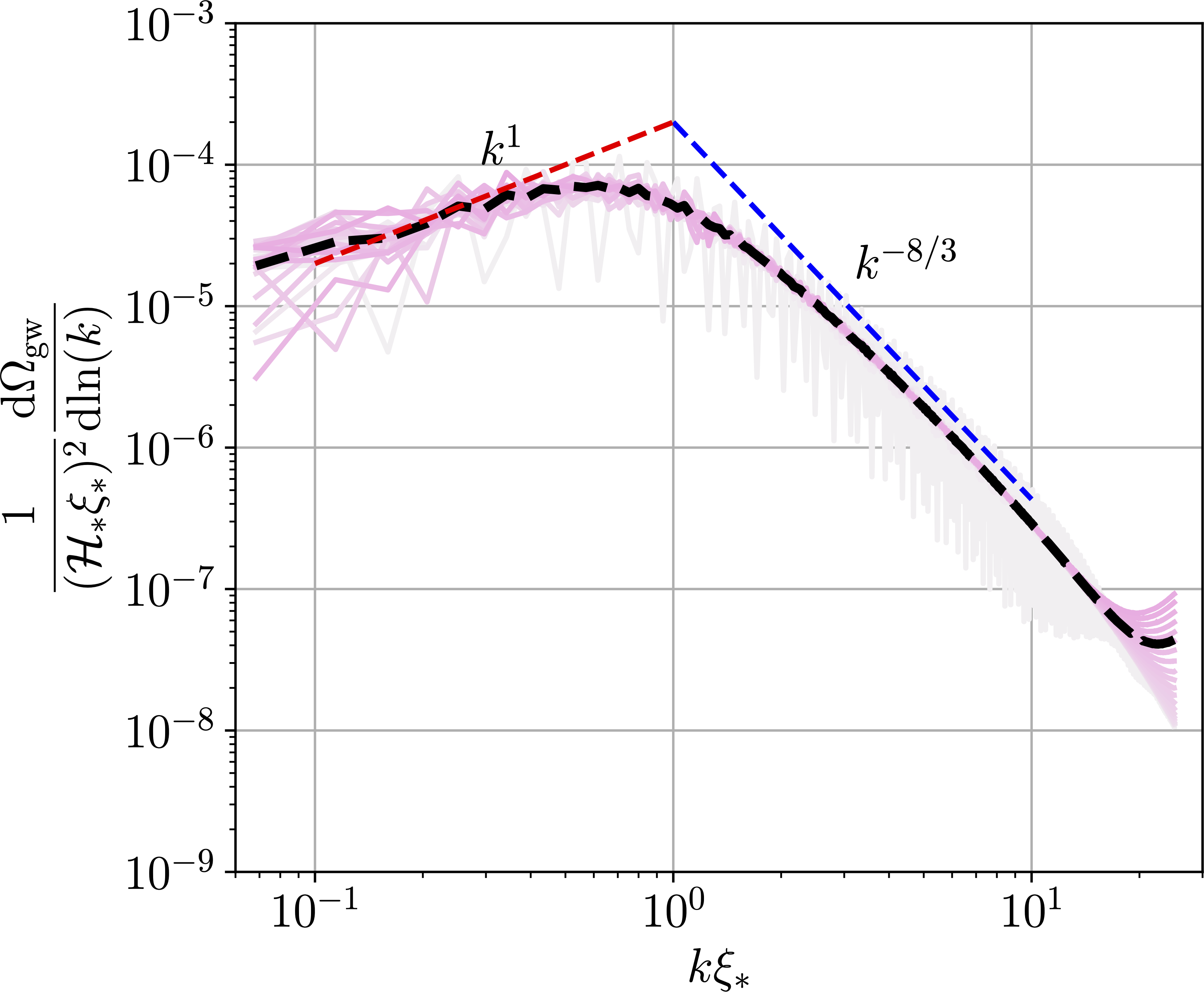
Sound waves ➤ acoustic turbulence
- Thermal phase transitions produce sound waves
- Over time, sound waves steepen into shocks
- Overlapping field of shocks = 'acoustic turbulence'
- Distinct from, but related to Kolmogorov turbulence
2d acoustic turbulence
Acoustic turbulence: GWs
Spectral shape $S$ as function of $k$ and integral scale $L_0$:
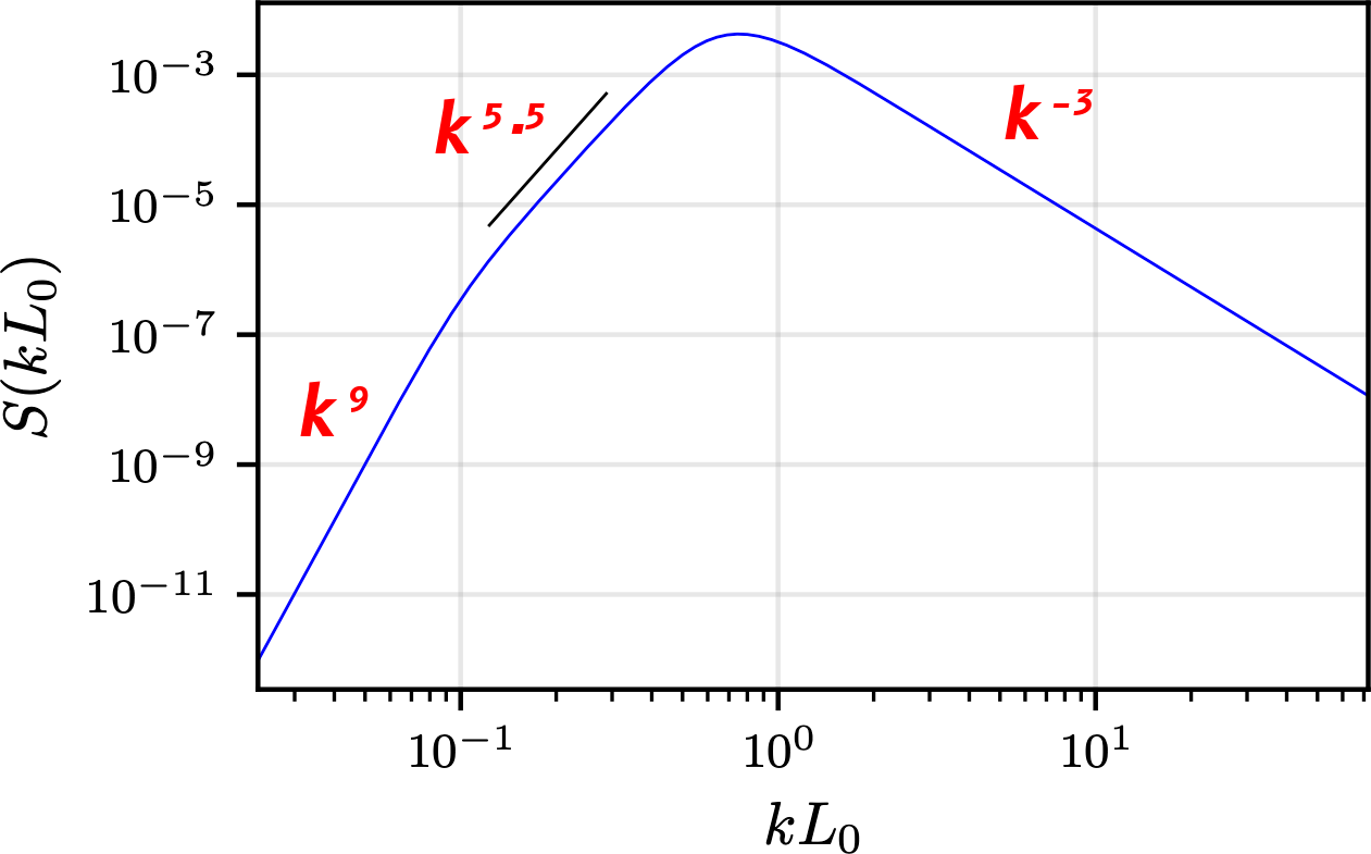
Different from sound waves and Kolmogorov turbulence!
⇒ all must be taken into consideration.
Kolmogorov turbulence: GWs
Validated theoretical modelling of GWs from Kolmogorov turbulence with large-scale simulations
The electroweak phase diagram, revisited
Remember this phase diagram?
- Simulate DR'ed 3D theory
on
lattice arXiv:hep-let/9510020
![]()
- With DR, can integrate out heavy new physics and study simpler model
When new physics is heavy
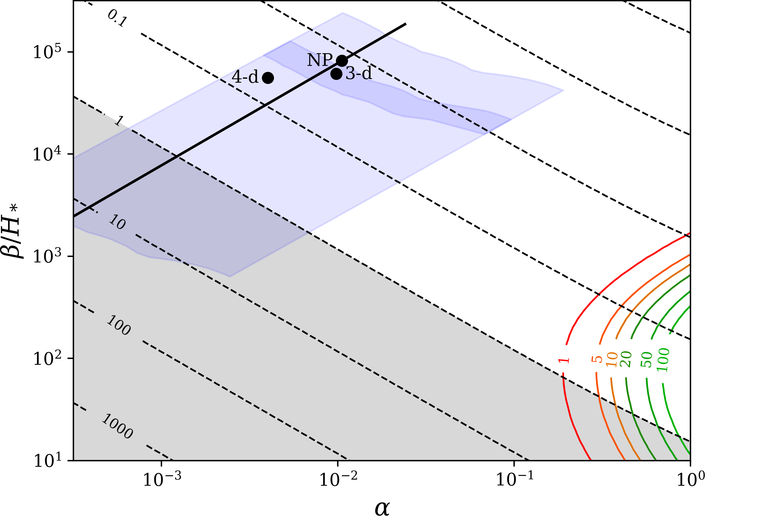
transition duration
- Comparison at benchmark point in minimal SM
- Compare: ● 4d PT vs ● 3d PT vs ● NP (= lattice)
How to get strong transitions?
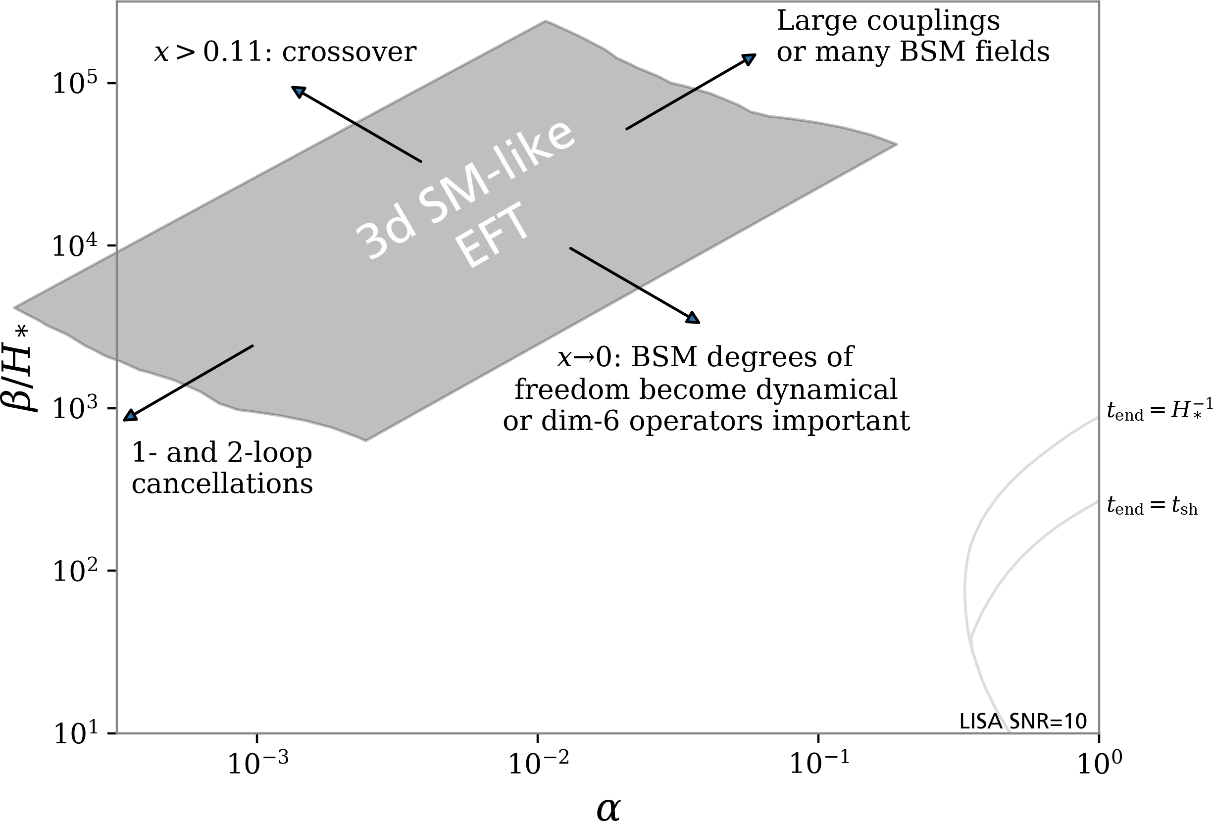
transition duration
- Theories that look SM-like in the IR ⇒ not observable!
- Then need additional light fields.
Wrapping up
Thanks
- Students:
Anna Kormu, Tiina Minkkinen, Mika Mäki, Riikka Seppä, Satumaaria Sukuvaara - Postdocs and researchers:
Jani Dahl, Deanna C. Hooper, - Collaborators past and present:
José Correia, Daniel Cutting, Oliver Gould, Jonathan Kozaczuk, Mark Hindmarsh, Stephan Huber, Lauri Niemi, Hiren Patel, Michael Ramsey-Musolf, Kari Rummukainen, Tuomas Tenkanen, Essi Vilhonen
Feedback...
... is very welcome!
- Please do fill in the feedback questionnaire!
- You can also email me, david.weir@helsinki.fi, with any questions or commments.
What I want you to remember
- Understanding primordial gravitational waves, even with my focus on phase transitions, involves many areas of physics, not just GR or cosmology.
- Early universe processes (such as phase transitions)
can probe and constrain BSM physics
... but we need precise predictions of key parameters $\Rightarrow$ lattice Monte Carlo simulations of phase transitions - Nonlinearities matter when studying phase transitions
$\Rightarrow$ large-scale real-time cosmological simulations