

Gravitational waves from thermal phase transitions,
from the bottom up
David J. Weir, University of Helsinki
Plan
- Introduction to EWPT
- Nucleation
- Wall velocities
- Thermodynamics
- Two approximations
- Simulations
- Models and predictions
1: Introduction to EWPT
Motivation
- Our aim is to study the non-equilibrium dynamics of the electroweak phase transition.
- EWPT connects the
biggest mysteries in modern physics:
- Baryogenesis and baryon asymmetry
- Origin of mass - Higgs mechanism
- Dark matter? Inflation? Neutrino masses?
- Difficult to probe the conditions of the EWPT at colliders.
- Hence use gravitational waves to see what happened!
Further reading
- On the electroweak model in
general:
Particle Data Book, Electroweak model review - On measuring the baryon
asymmetry:
Particle Data Book, Big Bang nucleosynthesis review - On electroweak
baryogenesis:
Morrissey and Ramsey-Musolf; Cline lectures
Baryon asymmetry of the universe
- Everyday experience: more baryons than antibaryons
- Quantify this through the asymmetry parameter $$ \eta = \frac{n_B - n_\overline{B}}{n_\gamma}$$
- From Planck, we have $\eta = (6.10 \pm 0.04) \times 10^{-10}$ excess baryons per photon
- This sounds small... but it's not!
Deriving $\eta$
- $\Omega_\mathrm{B} h^2 = 0.02207 \pm 0.00033 = \rho_\mathrm{b}/\rho_\mathrm{crit}$
- Then $$\eta = \frac{\rho_\mathrm{crit} \Omega_\mathrm{B}}{\langle m \rangle n_\gamma}.$$
- And from the Friedmann equation $$\rho_\mathrm{crit} = \frac{3 H_0^2}{8 \pi G}.$$
- Photon number density today $$n_\gamma = 2 \zeta(3) T_0^3 / \pi^2$$
- Mean mass per baryon $\langle m \rangle \approx m_\mathrm{p}$ (but smaller due to Helium binding)
Sakharov conditions
- Assume $B=0$ when the universe was created; $B>0$ later.
- In 1967 Andrei Sakharov (implicitly) wrote down the
necessary (but not sufficient) conditions for baryogenesis:
- Baryon number $B$ violation
- $C$ and $CP$ violation
- Departure from thermal equilibrium
- These specify only what is needed, not how it works.
More on the Sakharov conditions: $C$
- Note that if we had $B$ violation without $C$ violation, then $\overline{B}$ violation would occur at the same rate: $$ \Gamma(X \to Y + B) = \Gamma(\overline{X} \to \overline{Y} + \overline{B}) $$
- Thus over time $B=0$ still, unless we have $C$ violation too: $$ \frac{\mathrm{d} B}{\mathrm{d} t} \propto \Gamma(\overline{X} \to \overline{Y} + \overline{B}) - \Gamma(X \to Y + B).$$
More on the Sakharov conditions: $CP$
- In fact, also need $CP$ violation
- Consider $B$-violating $X \to q_\mathrm{L} q_\mathrm{L}$ process making left handed baryons
- $CP$ symmetry turns this equation into $ \bar{X} \to \bar{q}_\mathrm{R} \bar{q}_\mathrm{R}$
Electroweak baryogenesis
Kuzmin, Rubakov, Shaposhnikov
- Assume that there was no net baryon charge before the $\mathrm{SU}(2)_L \times \mathrm{U}(1)_Y \to \mathrm{U}(1)_\text{EM}$ breaking
- Processes that take place as the Higgs boson becomes massive responsible for creating a net baryon number
- Basically needs a first order phase transition to be successful (exceptions exist)
- Baryons produced through the anomaly $$ \begin{multline} B(t) - B(0) = 3[N_\text{cs}(t) - N_\text{cs}(0)]\\ = 3\int \mathrm{d} t \int \mathrm{d}^3x \frac{1}{16 \pi^2} \mathrm{Tr} \, F_{\mu\nu} \tilde{F}^{\mu\nu}. \end{multline}$$
Illustration
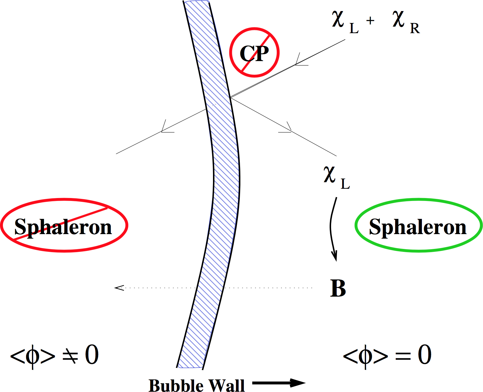
EW BG and the Sakharov conditions
Electroweak baryogenesis satisfies the Sakharov conditions:- $C$ and $CP$ violation: occurs due to particles scattering off bubble walls
- $B$ violation: the $C$ and $CP$ violation means that sphaleron transitions in front of the wall produce more baryons than antibaryons
- Out of equilibrium: the bubble walls (and sound shells) disturb the symmetric-phase equilibrium state
EW PT in the SM
Work in the 1990s found this phase diagram for the SM:
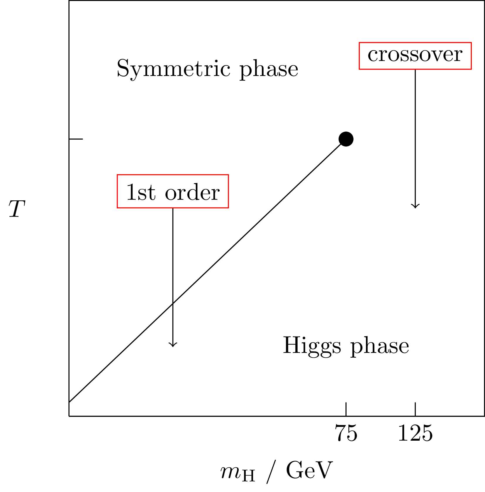
At $m_H = 125 \, \mathrm{GeV}$, SM is a crossover
Kajantie et
al.; Gurtler et al.;
Csikor et al.;
...
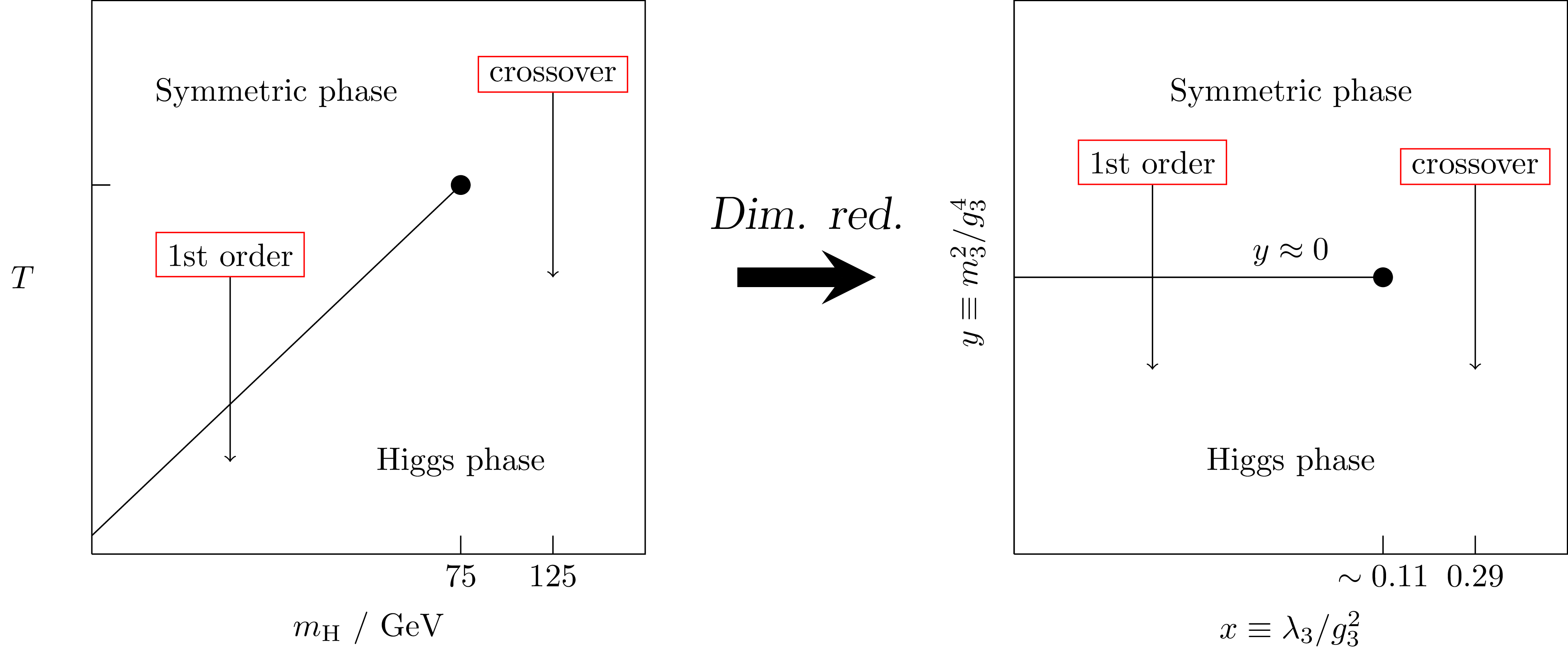
Dimensional reduction
- At high $T$, system looks 3D for long distance
physics
(with length scales $\Delta x \gg 1/T$) - Decomposition of fields: $$ \phi(x,\tau) = \sum_{n=-\infty}^{\infty} \phi_n(x) e^{i \omega_n \tau}; \qquad \omega_n = 2n\pi T $$
- Then integrate out $n\neq 0$ Matsubara modes due to the scale separation $$ \begin{align} Z & = \int \mathcal{D} \phi_0 \mathcal{D} \phi_n e^{-S(\phi_0) - S(\phi_0, \phi_n)} \\ & = \int \mathcal{D} \phi_0 e^{-S(\phi_0) - S_\text{eff}(\phi_0)} \end{align}$$
- The 3D theory (with most fields integrated out) is easier to study, has fewer parameters!
Using the dimensional reduction
- Using the DR'ed 3D theory, can study nonperturbatively with lattice simulations.
- This was done very successfully in the 1990s for the
Standard Model:
![]()
- [Q: Can we map any other theories to the same 3D model?]
SM is a Crossover
At $m_H = 125 \, \mathrm{GeV}$, critical temperature is $159.5 \pm 1.5 \, \mathrm{GeV}$
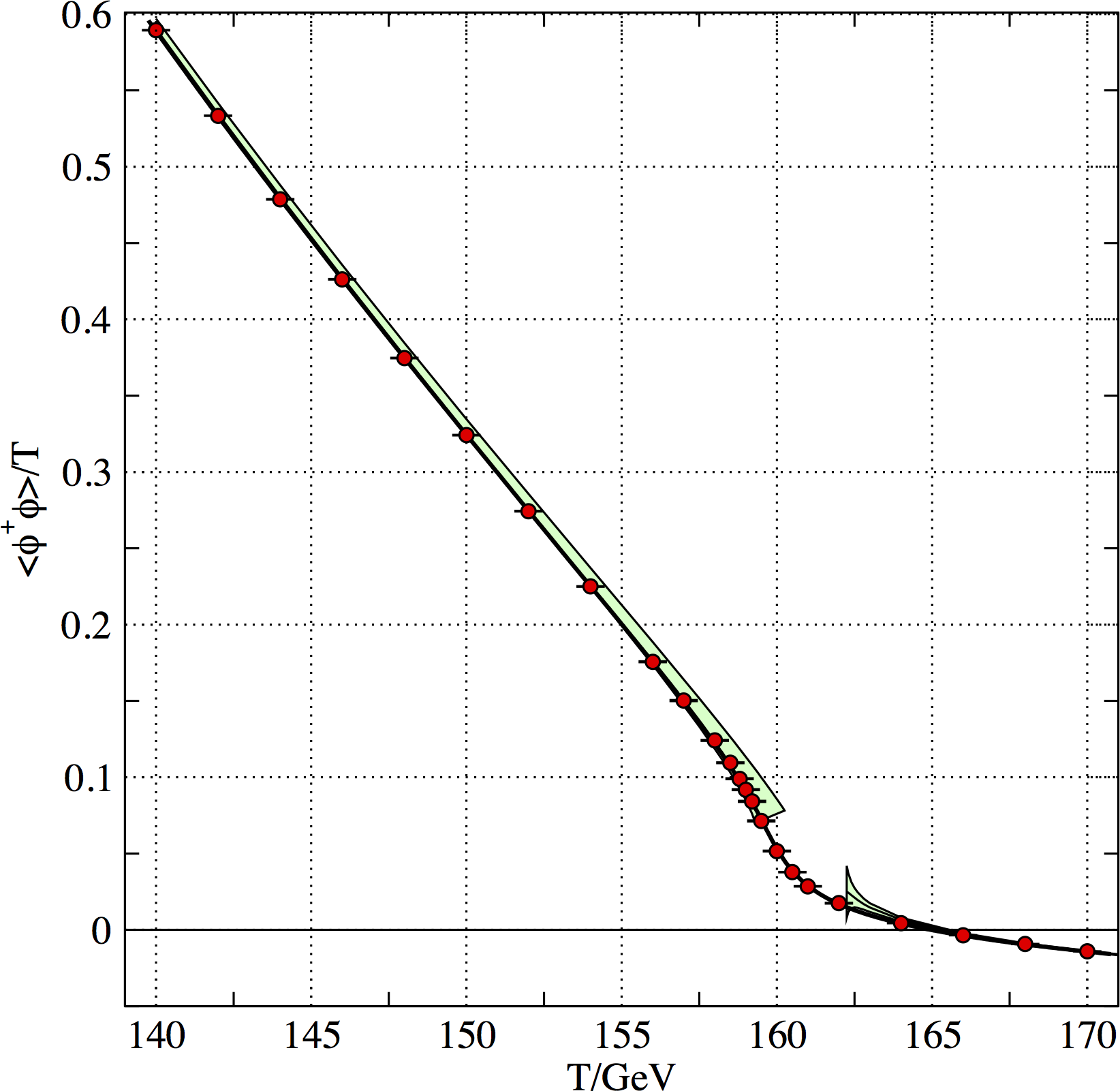
Source: D'Onofrio and Rummukainen
SM is a crossover: consequences
- No real departure from thermal equilibrium
⇒ no significant GWs or baryogenesis - Many alternative mechanisms for baryogenesis exist
- Leptogenesis (add RH neutrinos, see-saw mechanism, additional leptons produced by RH neutrino decays)
- Cold electroweak baryogenesis (non-equlibrium physics given by supercooled initial state)
SM extensions with 1PT
- Higgs singlet model - add extra real singlet field $\sigma$: quite difficult to rule out with colliders
- Two Higgs doublet model - add second complex doublet (like the Higgs): many parameters, but already quite constrained
- Triplet models - add adjoint scalar field (triplet): few parameters, not yet widely studied
All these have unexcluded regions of parameter space for which the phase transition is first order (and for which EW BG may be possible)
Higgs singlet model
$$ \mathcal{L}_{\Phi,\sigma} = D_\mu \phi^\dagger D_\mu\phi-\mu_h^2\phi^\dagger\phi+\lambda_h(\phi^\dagger\phi)^2+\frac{1}{2}(\partial_\mu\sigma)^2+\frac{1}{2}\mu_\sigma^2\sigma^2\\ +\mu_1\sigma+\frac{1}{3}\mu_3\sigma^3+\frac{1}{4}\lambda_\sigma\sigma^4+\frac{1}{2}\mu_m\sigma\phi^\dagger\phi+\frac12\lambda_m\sigma^2\phi^\dagger\phi$$
- More complicated symmetry breaking: $\sigma$, $\phi$ can get vevs...
- Singlet doesn't couple to gauge fields, harder to see at LHC
- If singlet is heavy, we can integrate it out during DR
- Then we rule out regions of parameter space where it
plays an active role, but:
- Some of that is at light singlet masses (and hence disfavoured) anyway
- The system then maps onto the same 3D theory as the Standard Model! Two potential parameters: $x$, $y$
Higgs singlet model
Nb: $\lambda_m = 2 \lambda_\mathrm{HS}$
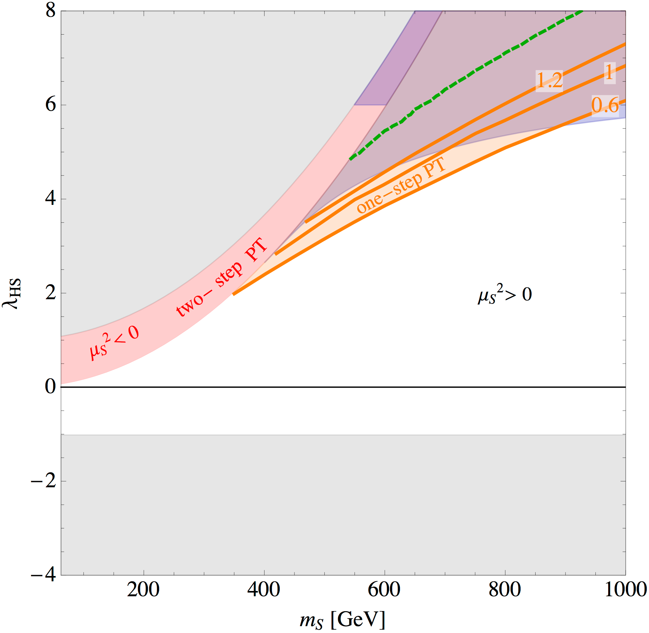
Source: Curtin, Meade and Yu
Two Higgs doublet model

Two Higgs doublet model
- Scalar Lagrangian: $ \mathcal{L}_\text{scalar}= (D_\mu\phi_1)^\dagger (D_\mu\phi_1) + (D_\mu\phi_2)^\dagger (D_\mu\phi_2) $ $ + \rho (D_\mu\phi_1)^\dagger (D_\mu\phi_2) + {\rho}^* (D_\mu\phi_2)^\dagger (D_\mu\phi_1) + V(\phi_1, \phi_2)$
- Potential: $V(\phi_1,\phi_2) = \mu^2_{11} \phi_1^\dagger \phi_1 + \mu^2_{22} \phi_2^\dagger \phi_2 + \mu^2_{12} \phi_1^\dagger \phi_2 + \mu^{2*}_{12} \phi_2^\dagger \phi_1$ $ + \lambda_1 (\phi_1^\dagger \phi_1)^2 + \lambda_2 (\phi_2^\dagger \phi_2)^2 + \lambda_3 (\phi_1^\dagger \phi_1)(\phi_2^\dagger \phi_2) $ $ + \lambda_4 (\phi_1^\dagger \phi_2)(\phi_2^\dagger \phi_1) + \frac{\lambda_5}{2} (\phi_1^\dagger \phi_2)^2 + \frac{\lambda^*_5}{2} (\phi_2^\dagger \phi_1)^2 $ $ + \lambda_6 (\phi_1^\dagger \phi_1)(\phi_1^\dagger \phi_2) + \lambda^*_6 (\phi_1^\dagger \phi_1)(\phi_2^\dagger \phi_1) $ $ + \lambda_7 (\phi_2^\dagger \phi_2)(\phi_2^\dagger \phi_1) + \lambda^*_7 (\phi_2^\dagger \phi_2)(\phi_1^\dagger \phi_2). $
Two Higgs doublet model
- Lots of parameters, but extensively studied already.
- Because it couples directly to the gauge fields, it is easier to observe than a real singlet.
Higgs triplet model
- A bit simpler: $$ \mathcal{L}_\text{scalar}= (D_\mu\phi)^\dagger (D_\mu\phi) + \frac12 D_\mu \Sigma^a D_\mu \Sigma^a + V(\phi, \Sigma) $$ with potential $$ V(\phi,\Sigma) = \mu^2_{\phi} \phi^\dagger \phi + \lambda (\phi^\dagger \phi)^2 \\ +\frac{1}{2} \mu^2_\Sigma \Sigma^a \Sigma^a + \frac{b_4}{4} (\Sigma^a \Sigma^a)^2 + \frac{a_2}{2} \phi^\dagger \phi \Sigma^a \Sigma^a. $$
- Again, $\Sigma$ couples to gauge field
⇒ triplet should already have been seen...
A big caveat
- The above models have only been extensively studied in perturbation theory.
- In coming months and years the viability of first-order phase transitions will be tested with non-perturbative methods.
- As a rule, non-perturbative methods indicate that phase transitions are weaker than expected, but not always!
PT vs. non-perturbative
MSSM ('light stop'): transition stronger on lattice
Source: Laine, Nardini and Rummukainen
Intro to EPWT - conclusion
- SM is a crossover
- Many simple extensions with first order phase transitions
- Will take a next-generation collider (or GW detection!) to rule out most models
- And need new simulations to pin down the likely parameter space
2: Nucleation
Motivation
- We now know that models exist which have a first-order phase transition at the electroweak scale.
- How do we study bubble collisions in these models?
- First step: how do bubbles form?
Motivation

CC-BY-SA by cyclonebill, from Wikimedia commons
Motivation
- Basic goal: calculate probability of a droplet of new phase appearing in a system made up entirely of the old phase
- Details depend somewhat on temperature:
- At zero temperature - quantum process
- At high temperature - thermal process
- Rate of nucleation important for determining whether phase transition will complete
- Nucleation rate a key factor in determining GW power spectrum amplitude
Further reading
- The only nonperturbative calculation: Moore and Rummukainen
- Basic idea: Langer
- Nucleation rates and the phase transition duration:
Enqvist, Ignatius, Kajantie and Rummukainen (see also Kapusta)
Nucleation basics
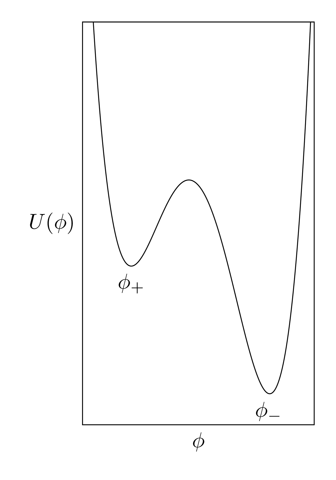
- When the universe drops below the critical temperature, broken phase is the new global minimum.
- Quantum (or thermal) fluctuations will excite the field over the potential barrier to the new minimum.
- Consider a single scalar field $\phi$ with Lagrangian $$ \mathcal{L} = \frac{1}{2} \partial_\mu \phi \partial^\mu \phi - U(\phi) $$ and equation of motion $$ \frac{\partial^2 \phi}{\partial t^2} + \nabla^2 \phi = U'(\phi).$$
More nucleation basics
- Want to calculate probability for field $\phi$ to tunnel from false vacuum $\phi_+$ to true vacuum $\phi_-$.
- Like calculating a tunnelling amplitude in quantum mechanics.
- Solve for trajectory that 'bounces' from $\phi_+$ to $\phi_-$ and back again in a localised region
- This will give the exponential factor in the nucleation probability.
Computing the bounce
- At $T=0$, system has $\mathrm{O}(4)$ invariance, so change variables to $\rho = \sqrt{t^2 + \mathbf{x}^2}$: $$ \frac{\mathrm{d}^2 \phi}{\mathrm{d} \rho^2} + \frac{3}{\rho} \frac{\mathrm{d} \phi}{\mathrm{d} \rho} = U'(\phi).$$ with boundary conditions $$ \begin{align} \lim_{\rho \to \infty} \phi(\rho) & = \phi_+ \\ \left. \frac{\partial \phi}{\partial_\rho} \right|_{\rho=0}& =0 \end{align} $$
- Solve this by shooting, and then compute the action $S_4$ for this path.
Fluctuations and finite temperature
- Add a prefactor given by the contribution of fluctuations about the minimum $\phi_-$ and also the bounce path.
- However, we are interested in the finite-$T$ version of this calculation, in which case the symmetry is $\mathrm{O}(3)$.
- We can then use dimensional analysis to guess the prefactor: $$ \frac{\Gamma}{V} \approx T^4 \exp \left( -\frac{S_3(T)}{T} \right) $$ with $$ S_3 = 4\pi \int \mathrm{d}r \, r^2 \left[ \frac{1}{2} \left( \frac{d \phi}{d r} \right)^2 + V_\text{eff}(\phi, T) \right]. $$
Nucleation rates
- The full (finite-T) expression is $$ \begin{multline}\frac{\Gamma}{V} = \frac{\omega_-}{\pi} \left(\frac{S_3}{2\pi T} \right)^{3/2} \left[ \frac{\mathrm{det'}\left[ -\nabla^2 + V''(\phi_-, T)\right]}{\mathrm{det} \left[ -\nabla^2 + V''(\phi_+,T)\right] } \right]^{-1/2} \\ \times \exp \left( - \frac{S_3(T)}{T} \right). \end{multline} $$
- The above expression is very similar to that for the sphaleron rate - the two processes have much in common
Limiting cases for $S_3$
- As discussed above, solve for bounce profile by shooting.
- Identify two limiting cases:
- For small supercooling ($T_\mathrm{c} - T_N \ll T_\mathrm{c}$), bubbles are thin-wall type (with $\tanh$ walls).
- For large supercooling, bubbles are close to a Gaussian.
Beyond $S_3$
- Using $S_3(T)/T$ as the exponential parameter in the nucleation rate is a high-temperature approximation.
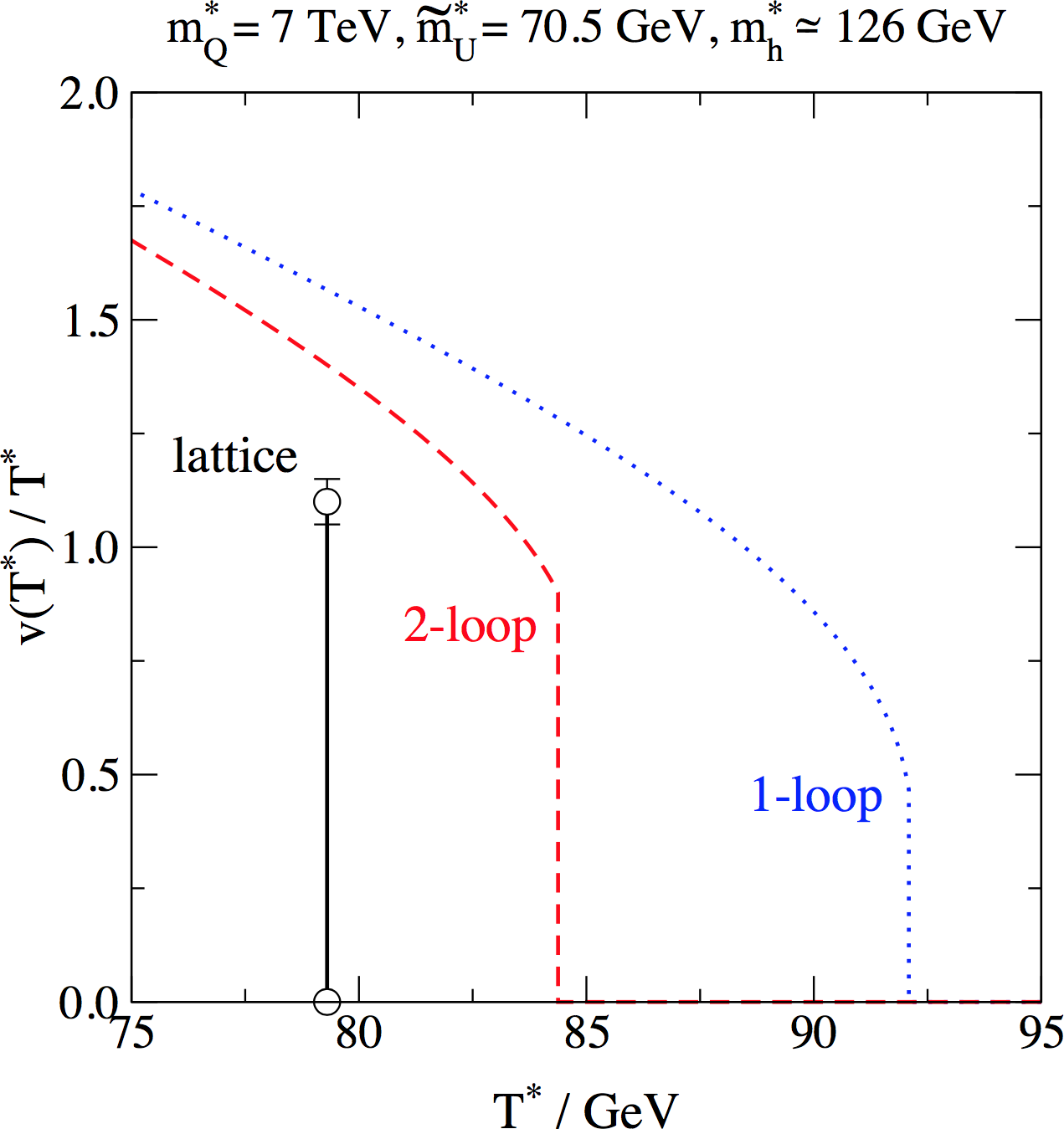
- One can also compute the nucleation rate
nonperturbatively, both the prefactor and the
exponential part. Results suggest that (for SM):
- True supercooling lies between 1- and 2-loop results
- 2-loop perturbative surface tension close to true result
- Unfortunately, nucleation rate only studied at one point in the dimensionally reduced SM theory - so generally still follow the usual anaysis
Making use of $\Gamma$
- The nucleation rate $\Gamma$ gives the probability of nucleating a bubble per unit volume per unit time.
- More useful for cosmology is to consider the inverse duration of the phase transition, defined as $$ \beta \equiv - \left.\frac{d S(t)}{d t} \right|_{t=t_*} \approx \frac{\dot \Gamma}{\Gamma} $$
- The phase transition completes when the probability of nucleating one bubble per horizon volume is of order 1 $$ S_3(T_*)/T_* \sim -4 \log \frac{T_*}{m_\mathrm{Pl}} \approx 100 $$
Making further use of $\Gamma$
- Using the adiabaticity of the expansion of the universe the time-temperature relation is $$ \frac{d T}{d t} = - T H $$
- This gives, for the ratio of the inverse phase transition duration relative to the Hubble rate, $$ \frac{\beta}{H_*} = T_* \left. \frac{dS}{dT} \right|_{T = T_*} = T_* \frac{d}{d T} \left. \frac{S_3(T)}{T} \right|_{T=T_*}$$
- If $\frac{\beta}{H_*} \lesssim 1$ then the phase transition won't complete...
Nucleation - conclusion
- Nucleation rate per unit volume per unit time $\Gamma$ computed from bounce actions $S(T) = \mathrm{min}\{ S_3(T)/T ,S_4(T) \}$
- Inverse duration relative to Hubble rate $\frac{\beta}{H_*}$ computed from $\Gamma$, and controls GW signal
- To get $\beta$:
- Find effective potential $V_\text{eff}(\phi,T)$
- Compute $S_3(T)/T$ (or $S_4(T)$) for extremal bubble by solving 'equation of motion'
- Determine transition temperature $T_*$
- Evaluate $\beta/H$ at $T_*$
- Use $\beta/H_*$ as input to the GW power spectrum.
3: Wall velocities
Motivation
- Wall velocity connects the electroweak phase
transition to the two big unknowns:
- Baryogenesis (rate of baryon asymmetry production)
- Gravitational waves ($v_\text{wall}^3$ dependence)
- [Almost] at the bottom of a hierarchy of abstraction:
- Can derive friction term for higher-level simulations
- Check how valid using a single scalar field and ideal fluid really is.
Further reading
- Prokopec and
Moore: hep-ph/9503296
and hep-ph/9506475. - Konstandin, Nardini and Rues: arXiv:1407.3132.
- Kozaczuk: arXiv:1506.04741.
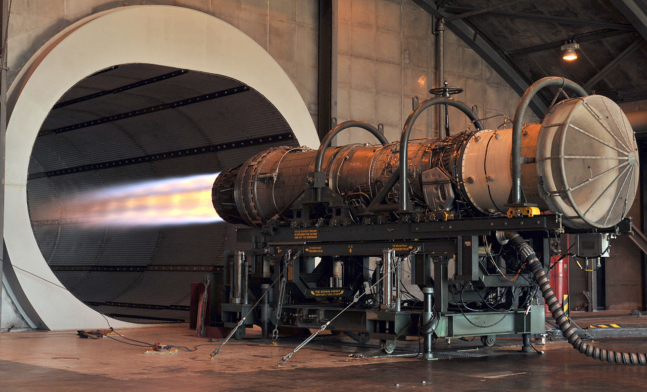
What happens at the bubble wall?
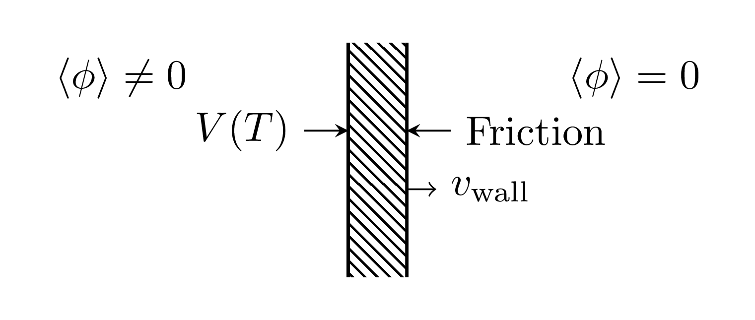
- Forces in equilibrium:
- Inside, $\langle \phi \rangle \neq 0$, latent heat $\mathcal{L} = \Delta V(T)$ released.
- Outside, $\langle \phi \rangle = 0$, friction from everything coupling to $\phi$.
- When there is no net force, wall stops accelerating.
- Is there a finite $v_\text{wall}$ below $c$ for which this happens?
- (Vacuum case: no force on wall - nothing to stop it accelerating to $c$)
Free body diagram
What does the friction term look like?
- Expand Higgs field about classical profile $$\Phi(x,t) \to \Phi_\mathrm{cl}(x,t) + \delta \Phi(x,t)$$ and follow behaviour of $\Phi_\mathrm{cl}$.
- In the Standard Model, equation of motion is
$ \partial_\mu \partial^\mu \Phi_\mathrm{cl} - \mu \Phi_\mathrm{cl} + 2 \lambda (\Phi^\dagger_\mathrm{cl} \Phi_\mathrm{cl})\Phi_\mathrm{cl} \\ + 2 \lambda \left( 2 \langle \delta \Phi^\dagger \delta \Phi \rangle \Phi_\mathrm{cl} + \langle \delta \Phi^2 \rangle \Phi_\mathrm{cl}^\dagger \right) - \frac{g^2}{4} \langle A^2 \rangle + \sum y \langle \overline\psi_\mathrm{R} \phi_\mathrm{L} \rangle = 0$
- Top line - classical bits; bottom line - fluctuations
- How to treat the fluctuations?
Consider one component $\phi$ from $\Phi = (0,\phi/\sqrt{2})$ ...
- Field $\phi$ is slowly varying compared to
reciprocal momenta of particles in plasma ($\propto
T$)
⇒ treat in WKB - Write phase space density as $f(\mathbf{k},\mathbf{x})$
- Separate into equilibrium and nonequilibrium
parts, $ f(\mathbf{k},\mathbf{x}) \to f(\mathbf{k}, \mathbf{x}) + \delta f(\mathbf{k},\mathbf{x}) $
- $f(\mathbf{k}, \mathbf{x})$ due to equilibrium thermal fluctuations; absorbed into 'finite-temperature effective potential' for $\Phi_\mathrm{cl}$
- $\delta f(\mathbf{k}, \mathbf{x})$ is the departure from that equilibrium
- Equation of motion is (schematically)
$$ \partial_\mu \partial^\mu \phi + V_\text{eff}'(\phi,T) +
\sum_{i} % \in \text{massive ds.o.f.}}
\frac{d m_i^2}{d \phi} \int
\frac{\mathrm{d}^3 k}{(2\pi)^3 2 E_i} \delta f_i(\mathbf{k},\mathbf{x}) = 0$$
- $V_\text{eff}'(\phi)$: gradient of finite-$T$ effective potential
- $f_i(k,x)$: deviation from equilibrium phase space density of $i$th species
- $m_i$: effective mass of $i$th species:
- Leptons: $m^2 = y^2 \phi^2/2$
- Gauge bosons: $m^2 = g_w^2 \phi^2/4$
- Also Higgs and pseudo-Goldstone modes
After some algebra:
$$ \overbrace{\partial_\mu T^{\mu\nu}}^\text{Force on $\phi$} - \overbrace{\int \frac{d^3 k}{(2\pi)^3} f(\mathbf{k}) F^\nu }^\text{Force on particles}= 0 $$This equation is the realisation of this idea:
Another interpretation:
$$ \overbrace{\partial_\mu T^{\mu\nu}}^\text{Field part} - \overbrace{\int \frac{d^3 k}{(2\pi)^3} f(\mathbf{k}) F^\nu }^\text{Fluid part}= 0 $$i.e.:
$$ \partial_\mu T^{\mu\nu}_\phi + \partial_\mu T^{\mu\nu}_\text{fluid} = 0 $$We will return to this later!
Layers of abstraction
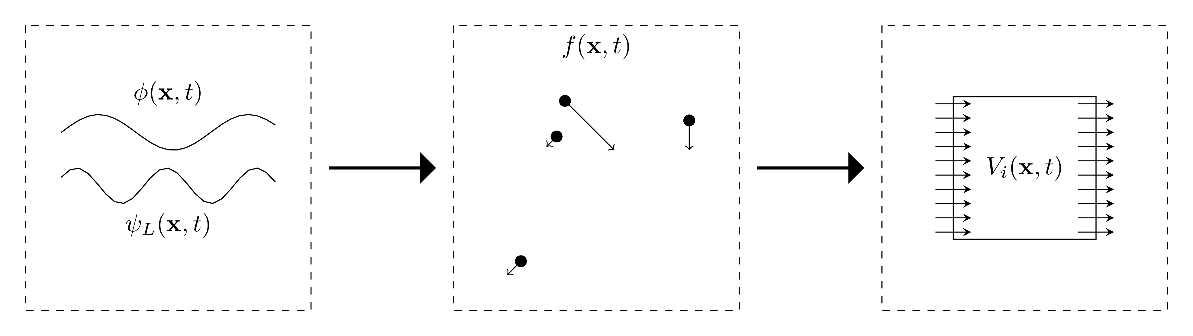
Layers of abstraction
- We have so far been using field theory equations of motion.
- Less tricky, but more abstract, are:
- Boltzmann equations
- Hydrodynamic equations
- In particular, the hydrodynamic equations we get are a valuable motivation for the rest of today's lectures
- We will now look at how to arrive at these higher-level approximations
Boltzmann equations: a reminder
What is a Boltzmann equation?
- Phase space is positions $\mathbf{x}$ and momenta $\mathbf{k}$.
- Tells us how our distribution functions $f_i(\mathbf{x},\mathbf{k})$ evolve.
- Consists of four parts:
- Time evolution $$\partial_t f_i(\mathbf{x},\mathbf{k}).$$
- Streaming terms in momentum and position space $$\dot{\mathbf{x}} \cdot \nabla_\mathbf{x} f + \dot{\mathbf{p}} \cdot \nabla_\mathbf{p} f$$
- Collision $$C[f]$$
Boltzmann equation for distribution $f$
- The Boltzmann equation is $$ \frac{\mathrm{d} f}{\mathrm{d} t} = \frac{\partial f}{\partial t} + \dot{\mathbf{x}} \cdot \nabla_\mathbf{x} f + \dot{\mathbf{p}} \cdot \nabla_\mathbf{p} f = -C[f].$$
- This is a semiclassical approximation to the quantum Liouville equations for all the fields
- Only valid when the momenta of the fields is much higher than the inverse wall thickness: $$ p \gtrsim g T \gg \frac{1}{L_w}. $$
- Very difficult to work with directly, so model the distribution $f_i$ of each particle with a 'fluid' ansatz.
Fluid approximation
- As mentioned, fluid approximation sets the scene for the rest of these lectures on the electroweak phase transition
- In short, we have $$ T_{\mu\nu}^\text{fluid} = \sum_i \int \frac{d^3 k}{(2\pi)^3 E_i} k_\mu k_\nu f_i(k) = w u_\mu u_\nu - g_{\mu\nu} p $$ but we will try to justify this.
Deriving the fluid approximation
- The flow ansatz is $$ f_i(k,x) = \frac{1}{e^X \pm 1} = \frac{1}{e^{\beta(x) ( u^\mu(x) k_\mu + \mu(x))} \pm 1} $$ with four-velocity $u^\mu(x)$, chemical potential $\mu(x)$ and inverse temperature $\beta(x)$.
- Substituting this ansatz into the Boltzmann equations for the system yields (after much algebra!) a (relativistic) Euler momentum equation $$ u^\mu \partial_\mu u_\nu + \partial_\nu p = C.$$
The field-fluid model
- Energy conservation requires that $$ \partial_\mu T^{\mu\nu} = \partial_\mu (T^{\mu\nu}_\phi + T^{\mu\nu}_\text{fluid}) = 0. $$
- We are now ready to present the full model: $$ \begin{align} (\partial_\mu \partial^\mu \phi) \partial^\nu \phi - \frac{\partial V_\text{eff}(\phi,T)}{\partial \phi} \partial^\nu \phi & = -\eta(\phi, v_\mathrm{w}) u^\mu \partial_\mu \phi \partial^\nu \phi \\ \partial_\mu (w u^\mu u^\nu) - \partial^\nu p + \frac{\partial V_\text{eff}(\phi,T)}{\partial \phi} \partial^\nu \phi & = + \eta(\phi, v_\mathrm{w}) u^\mu \partial_\mu \phi \partial^\nu \phi \end{align} $$
- Besides the (dimensionful) definition here, one choice for $\eta$ that is well motivated is $\tilde{\eta} \frac{\phi^2}{T}$.
- This model is the basis of spherical and 3D simulations. One can also obtain steady-state equations.
The field-fluid model: observations
- Consider the fluid equation: $$ \partial_\mu (w u^\mu u^\nu) - \partial^\nu p + \frac{\partial V_\text{eff}(\phi,T)}{\partial \phi} \partial^\nu \phi = \eta(\phi, v_\mathrm{w}) u^\mu \partial_\mu \phi \partial^\nu \phi $$
- Away from the bubble wall, the right hand side goes to zero. The left hand side has no length scale.
- Therefore any fluid solution must be parametrised by a dimensionless ratio, e.g. radius of the bubble to time since nucleation - define $\xi = r/t$.
- Fluid profiles will scale with the bubble radius: they are large, extended objects!
Runaway walls?
- We have assumed that the wall reaches a terminal velocity (less than $c$).
- But what if it doesn't? Termed a 'runaway wall'.
- Consequences would include:
- Less interaction with plasma
- Lower amplitude of GWs
- Runaway walls are currently a hot topic - with a recent paper suggesting that they may not exist (due to subleading corrections arising from the treatment of gauge bosons)
Wall velocities: conclusion
- Detailed studies have been carried out of the wall velocity, using thermal field theory techniques.
- Higher level calculations and simulations use an effective field-fluid model, with the wall velocity as an input parameter.
- The damping term for field-fluid models (and hence the wall velocity) is generally obtained by a qualitative matching to the Boltzmann equations.
4: Thermodynamics
Motivation
- In the previous section we described the various layers of approximation up to the field-fluid model.
- Now we will use that field-fluid model (and steady-state results) to explore the macroscopic behaviour of the wall.
- This is important both for baryogenesis and also for the GW power spectrum.
Further reading
- Energy budget: Espinosa, Konstandin, No and Servant arXiv:1004.4187
Combustion physics
Reaction front
- At a reaction front, there is a chemical transformation. The fluid is chemically and physically distinct on both sides.
- Different from a shock front, where the energy density and entropy change.
- We have a reaction front as $\langle \phi \rangle = 0$ before and $\langle \phi \rangle \neq 0$ after
Detonations vs deflagrations
- If the scalar field wall moves supersonically and the fluid enters the wall at rest, we have a detonation
- If the scalar field wall moves subsonically and the fluid enters the wall at its maximum velocity, we have a deflagration
- Can also get a hybrid where the wall moves supersonically but some fluid bunches up in front of it, like a deflagration
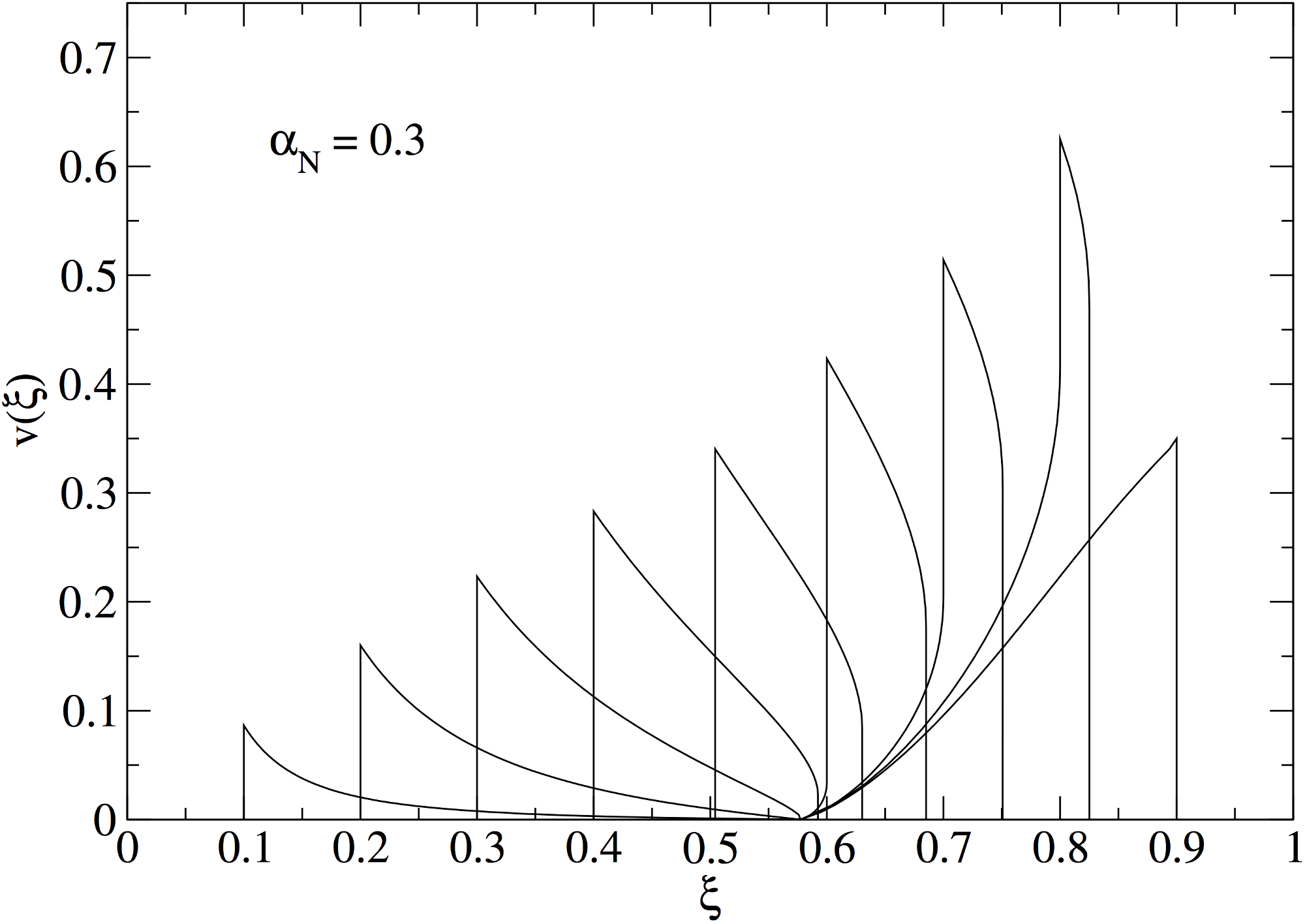
Fluid profile equation
- As mentioned before, away from the bubble wall, there is no length scale in the fluid equations.
- Therefore expect that fluid profile around a spherical bubble will scale as $\text{radius}/\text{time}$: $\xi = r/t$
- Rearrange Euler equation to remove diffusion, using $c_\mathrm{s} = \sqrt{(\mathrm{d}p/dT)(\mathrm{d}\epsilon/dT)}$
- Then, if we know the fluid velocity we can solve $$ 2 \frac{v}{\xi} = \gamma^2(1- v\xi)\left[\frac{\mu^2}{c_s^2} - 1 \right] \frac{\partial v}{\partial \xi} $$ with the Lorentz-boosted fluid velocity $ \mu(\xi, v) = (\xi - v)/(1 - \xi v). $
Fluid profiles
Phase transition strength
- The story so far:
- Bubbles nucleate (parameter $\beta$)
- Bubbles expand with finite velocity ($v_\mathrm{w}$)
- Extensive fluid shell around bubble
- Latent heat $\mathcal{L}$ turned into fluid KE???
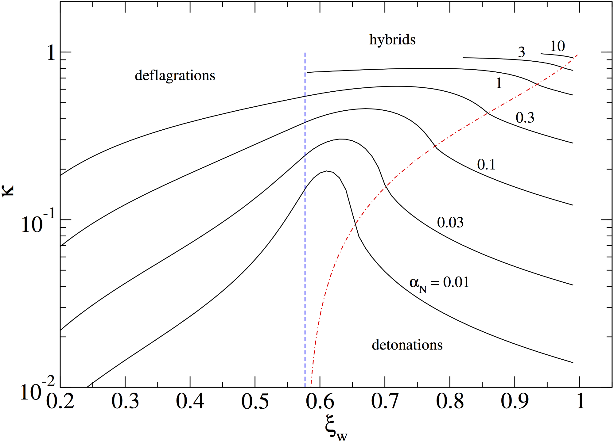
- Object of this section is to quantify how much of the latent heat ends up as kinetic energy.
- Define phase transition strength $$ \alpha_T = \frac{\mathcal{L(T)}}{g(T) \pi^2 T^4/30} = \frac{\text{latent heat at $T$}}{\text{radiation energy at $T$}} $$ which tell us how much of the energy of the universe was stored as latent heat in the phase transition.
Computing the efficiency
- Larger $\alpha_T$ ⇒ stronger phase transition
- But it does not tell us how much of $\mathcal{L}$ ends up as fluid kinetic energy
- For that we define the efficiency $$ \kappa_\mathrm{f} = \frac{w u_i u_i}{\mathcal{L}}= \frac{\text{fluid KE}}{\text{latent heat}}$$
- Then $\kappa_\mathrm{f} \alpha_T$ is the fraction of the energy density in the universe that ends up as fluid kinetic energy at the transition.
- Very roughly, $\kappa_\mathrm{f} \alpha_T \approx \overline{U}_f^2$, the Lorentz-boosted mean square fluid velocity as the transition completes.
- Can be computed more accurately either from spherical simulations or directly solving.
Efficiency curves
An aside: scalar field efficiency
- One can also define $$\kappa_\phi = \frac{\sigma}{\mathcal{L}} \frac{S}{V} = \frac{\text{scalar field gradients}}{\text{latent heat}} $$
- Note that because this scales as $S/V$, the surface area over the volume, this is suppressed by the inverse bubble radius.
- Hence for realistic thermal phase transitions, $\kappa_\phi$ is small.
Thermodynamics: conclusion
- Thermal first-order transitions have a reaction front
- Reaction fronts can be deflagrations (generally subsonic), detonations (supersonic) or hybrids (a mixture).
- The fluid reaches a scaling profile in $\xi = r/t$ based on the available latent heat and wall velocity.
- From this, one can compute the efficiency $\kappa_\mathrm{f}$ and hence how much of the energy in the universe ends up in the fluid $\kappa_\mathrm{f} \alpha_T$.
Recap
- What parameters have we introduced?
- EWPT introduction: latent heat
- Nucleation: inverse duration $\beta$
- Wall velocities: $v_\mathrm{w}$
- Thermodynamics: $\alpha_T$ and $\kappa$
- That more or less summarises what we need to know about the physics of the phase transition, so we can now talk about the production of GWs.
5: Two approximations
Motivation
- In this section we will briefly look at two widely-used but simple approximations.
- First, the quadrupole approximation makes a
reappearance.
- We will see why (a version of) the quadrupole formula is a bad approximation for bubbles
- The next approximation is the envelope
approximation
- This was widely used until recently for studying bubble collisions.
- It is still important for vacuum transitions where the scalar field walls are all that matters (and $\kappa_\phi$ can dominate)
Further reading
- "Weinberg formula" Weinberg
- Early quadrupole and envelope
calculations
[Kamionkowski and] Kosowsky and Turner [and Watkins] - Later envelope approximation results Huber and Konstandin
- Recent developments Jinno and Takimoto
Preliminaries
Starting point is the Weinberg formula $$ \frac{d E_\text{GW}}{d\omega \, d\Omega} = 2 G \omega^2 \Lambda_{ij,lm} (\hat{\bf{k}}) T_{ij}^* (\hat{\bf{k}}, \omega) T_{lm}(\hat{\bf{k}},\omega)$$ with $$ T_{ij} (\hat{\bf{k}}, \omega) = \frac{1}{2\pi} \int \mathrm{d}t \, e^{i\omega t} \int \mathrm{d}^3 x \, e^{-i\omega \hat{\bf{k}}\cdot \bf{x}} T_{ij}(\bf{x},t)$$ and $$ \Lambda_{ij,lm} \equiv P_{ij}(\hat{\bf{k}}) P_{lm}(\hat{\bf{k}}) - \frac{1}{2} P_{ij} (\hat{\bf{k}}) P_{lm}(\hat{\bf{k}}) $$ where $$ P_{ij}(\hat{\bf{k}}) = \delta_{ij} - \hat{\mathbf{k}}_i \hat{\mathbf{k}}_j $$Quadrupole approximation
- Consider a pair of vacuum scalar bubbles along the $z$-axis
- In integral for $T_{ij}$ take $\hat{\mathbf{k}}\cdot \mathbf{x} \to 0$, such that $$ T_{ij}(\hat{\mathbf{k}},\omega) \to T_{ij}^Q(\omega) \equiv \frac{1}{2\pi} \mathrm{d}t \, e^{i\omega t} \int \mathrm{d}^3 x \, T_{ij} (\mathbf{x},t) $$
- Using cylindrical symmetry... $$T_{ij}^Q (\omega) = T_{xx}^Q (\omega) + T_{yy}^Q (\omega) + T_{zz}^Q (\omega) = D(\omega) \delta_{ij} + \Delta (\omega) \delta_{iz} \delta_{jz}$$ where only $\Delta(\omega)$ sources gravitational waves.
Quadrupole approximation: result
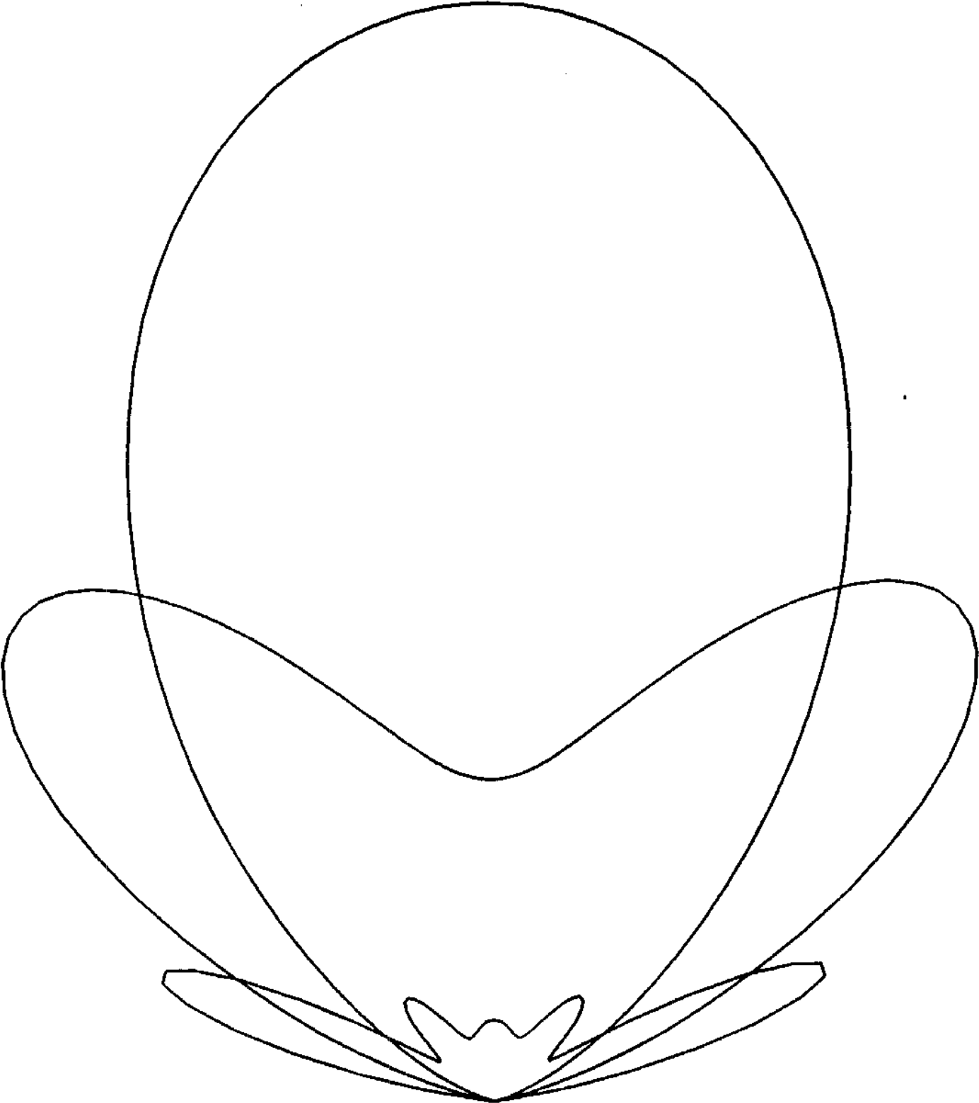
- Now note that
$$ \Lambda_{ij,lm} \delta_{iz} \delta_{jz} \delta_{lz}
\delta_{mz} = \Lambda_{zz,zz} = \frac{1}{2} \left( 1 -
\hat{\mathbf{k}}_z^2 \right)^2 = \frac{1}{2}\sin^4
\theta $$
![]()
- So, in the quadrupole approximation $$ \frac{\mathrm{d}E}{\mathrm{d}\omega \, \mathrm{d}\Omega} = G \omega^2 \left| \Delta(\omega) \right|^2 \sin^4 \theta $$
- Here $\Delta(\omega)$ can encode details of the bubble walls interacting, and can be found numerically.

O(2,1) simulation
Kosowsky, Turner and Watkins 1992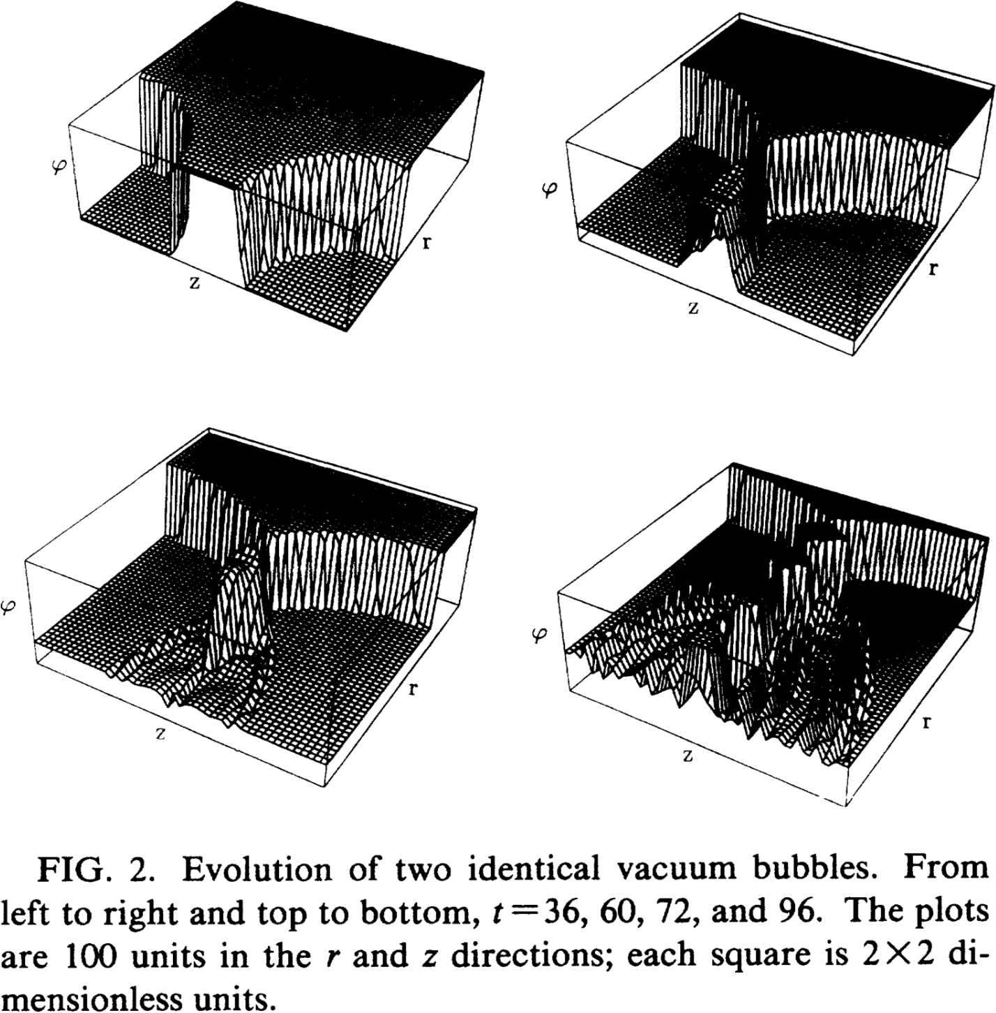
Limitations of the quadrupole approx.
Kosowsky, Turner and Watkins 1992![]() Quadrupole approximation is an overestimate!
Quadrupole approximation is an overestimate!-
Unfortunately at higher wavenumbers $\omega$, the
higher multipoles
dominate
- Only considered a pair of bubbles!
- In reality, many bubbles, less symmetry, bubble walls probably microscopic
- Motivates envelope approximation...
 Quadrupole approximation is an overestimate!
Quadrupole vs full linearised GR
Kosowsky, Turner and Watkins, 1992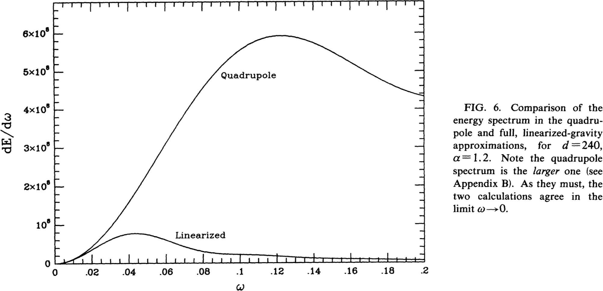
More about these early simulations:
- There is a nasty cutoff accounting for the $\mathrm{O}(2,1) $ symmetry
- Spacetime with $\mathrm{O}(2,1)$ symmetry is isomorphic to an $\mathrm{O}(3)$ pseudo-Schwarzschild-de Sitter spacetime
- Petrov type D - no GWs
Envelope approximation
Envelope approximation
Kosowsky, Turner and Watkins; Kamionkowski, Kosowsky and Turner- Thin, hollow bubbles, no fluid
- Stress-energy tensor $\propto R^3$ on wall
- Solid angle: overlapping bubbles → GWs
How is the envelope approximation implemented?
Envelope approximation: derivation
The stress energy tensor of the system $T_{ij}(\mathbf{x},t)$ can be turned into a sum of uncollided areas $S_n$ of each of the $n$ bubbles: $$ T_{ij}(\mathbf{k},\omega) = \frac{1}{2\pi} \int \mathrm{d} t \, e^{i\omega t} \sum_n \int_{S_n} \mathrm{d}\Omega \int \mathrm{d}r \, r^2 e^{-i\omega \hat{\mathbf{k}} \cdot (\mathbf{x}_n + r\hat{\mathbf{x}})} T_{ij,n}(r,t)$$ and then if we assume the walls are thin $$ 4 \pi \int \mathrm{d}r \, r^2 e^{-i\omega \hat{\mathbf{k}} \cdot (\mathbf{x}_n + r\hat{\mathbf{x}})} T_{ij,n}(r,t) \\ \approx \frac{4\pi}{3} e^{-i\omega \hat{\mathbf{k}} \cdot (\mathbf{x}_n + R_n(t) \hat{\mathbf{x}})} \hat{\mathbf{x}}_i \hat{\mathbf{x}}_j R_n(t)^3 \underbrace{\kappa \rho_\text{vac}}_{\text{i.e.}\, \sigma}.$$Envelope approximation: implementation
- With the approximation listed above, we get a double oscillatory integral: $$ \begin{align} T_{ij} (\hat{\mathbf{k}}, \omega) & = \kappa \rho_\text{vac} v_\mathrm{w}^3 C_{ij}(\hat{\mathbf{k}},\omega) \\ C_{ij} (\hat{\mathbf{k}},\omega) & = \frac{1}{6\pi} \sum_n \int \mathrm{d} t \, e^{i \omega(t -\hat{\mathbf{k}}\cdot \mathbf{x}_n)} (t-t_n)^3 A_{n,ij}(\hat{\mathbf{k}},\omega) \\ A_{n,ij}(\hat{\mathbf{k}},\omega) & = \int_{S_n} \mathrm{d} \Omega e^{- i \omega v_\mathrm{w} (t - t_n)\hat{\mathbf{k}}\cdot \hat{\mathbf{x}}} \hat{\mathbf{x}}_i \hat{\mathbf{x}}_j \end{align} $$
- Then evaluate these time-domain Fourier transforms numerically
- Integrate over uncollided areas $S_n$ at each timestep.
- Note that all $\hat{\mathbf{k}} \cdot \mathbf{x} \neq 0$, i.e. full result
Envelope approximation: implementation
Huber and Konstandin 2008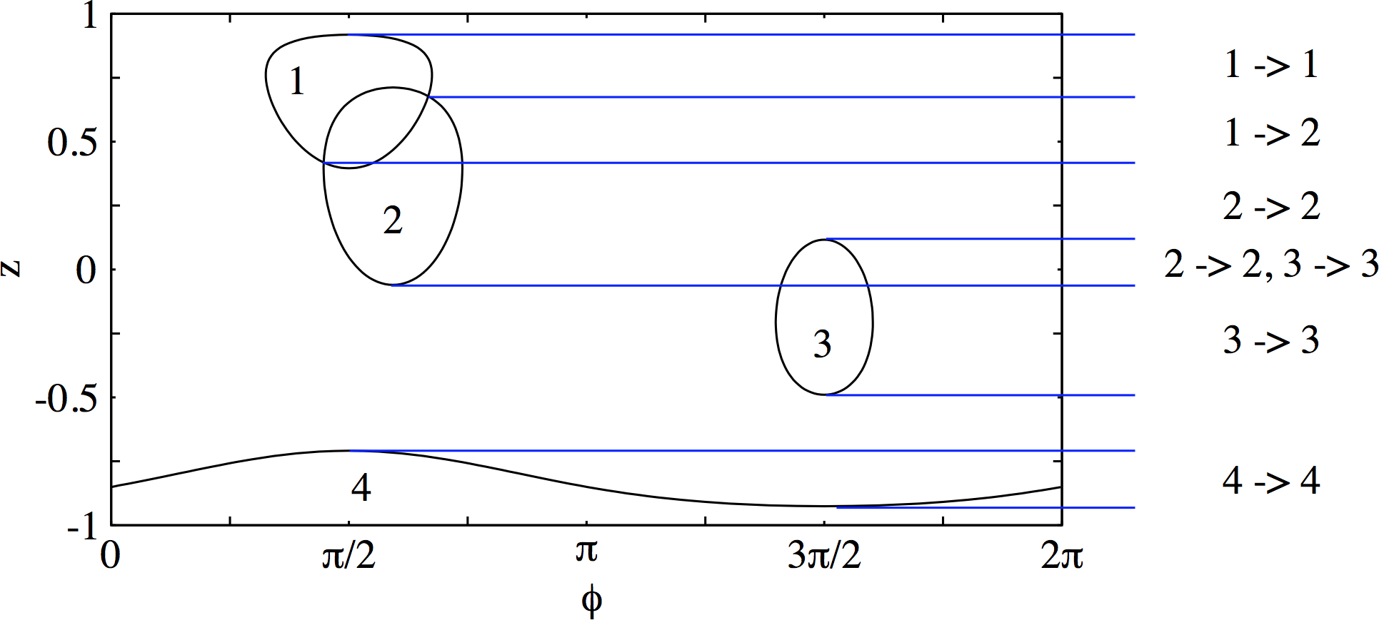
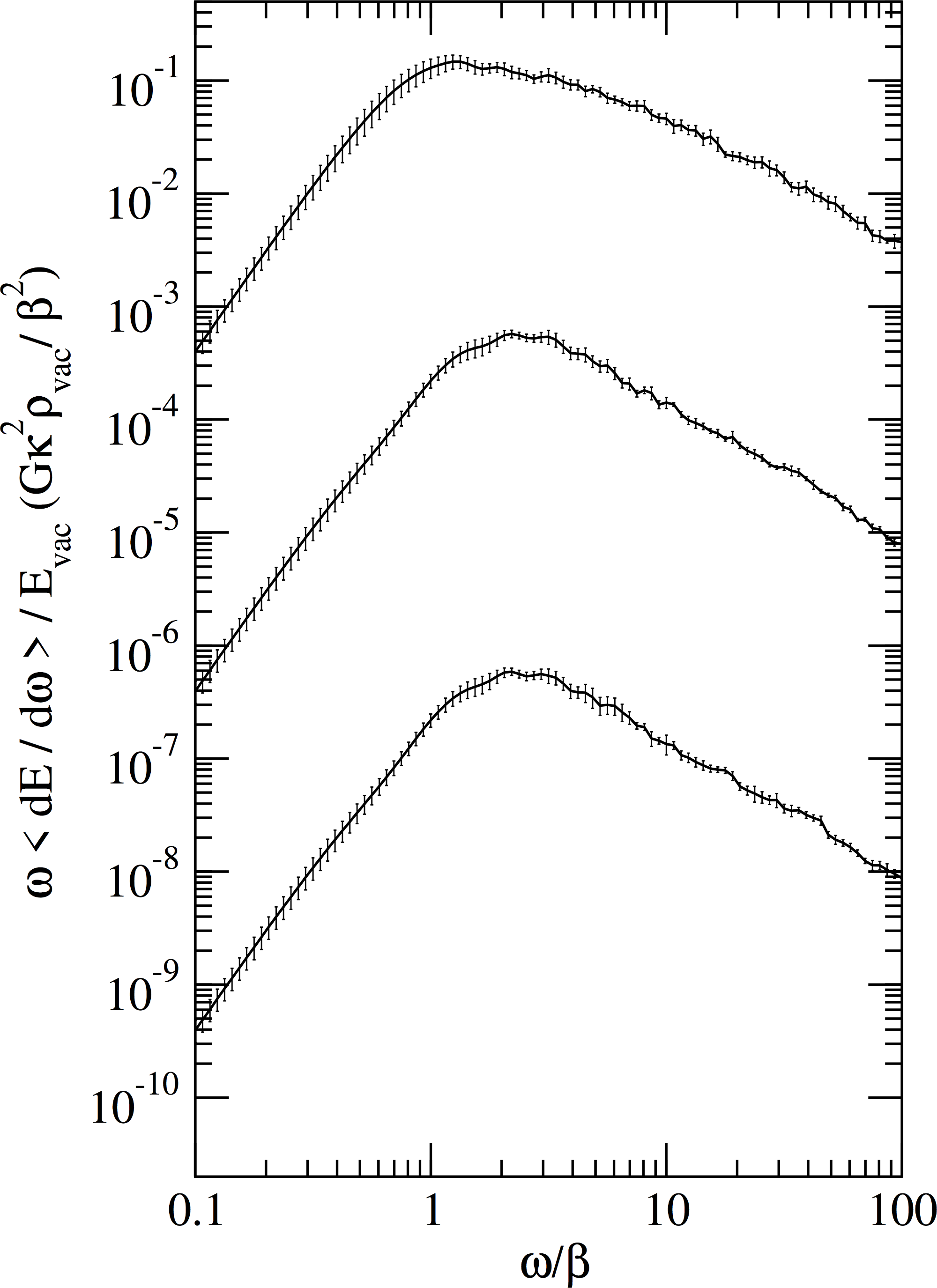
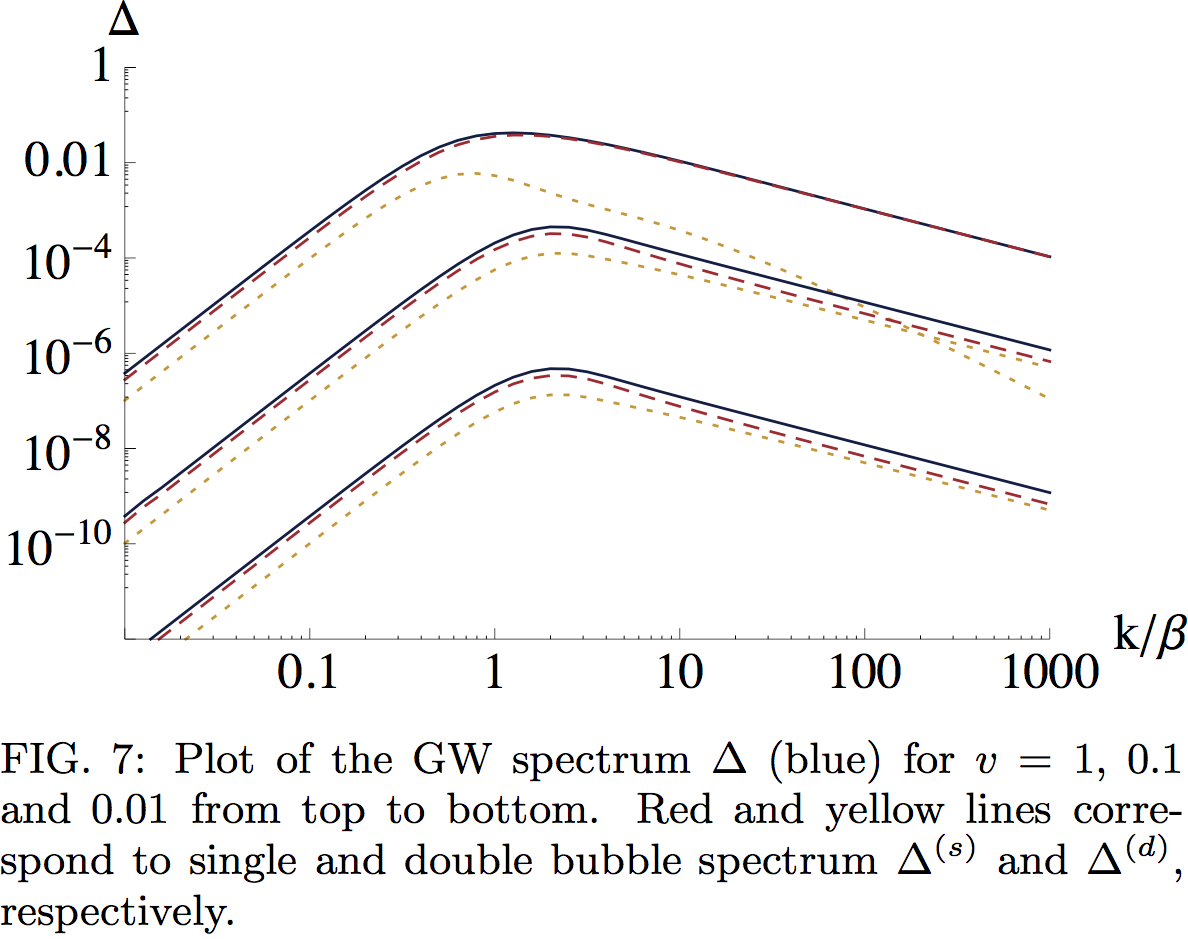
Envelope approximation: results
- Plot from Huber
and Konstandin 2008.
![]()
- Wall velocities top to bottom $v_\mathrm{w} = \{1,0.1,0.01\}$.
- Total power scales as $v_\mathrm{w}^3$.
- Peak at $\omega/\beta \approx 1$.
- Power laws on both sides of peak.
.jpg)
Envelope approximation: results
- Simple power spectrum:
- One length scale (average radius $R_*$)
- Two power laws ($\omega^3$, $ \sim \omega^{-1}$)
- Amplitude
NB: Used to be applied to shock waves (fluid KE),
now only use for bubble wall (field gradient energy)
Envelope approximation
4-5 numbers parametrise the transition:
- $\alpha_{T_*}$, vacuum energy fraction
- $v_\mathrm{w}$, bubble wall speed
- $\kappa_\phi$, conversion 'efficiency' into gradient energy $(\nabla \phi)^2$
- Transition rate:
- $H_*$, Hubble rate at transition
- $\beta$, bubble nucleation rate
[only matters for vacuum/runaway transitions]
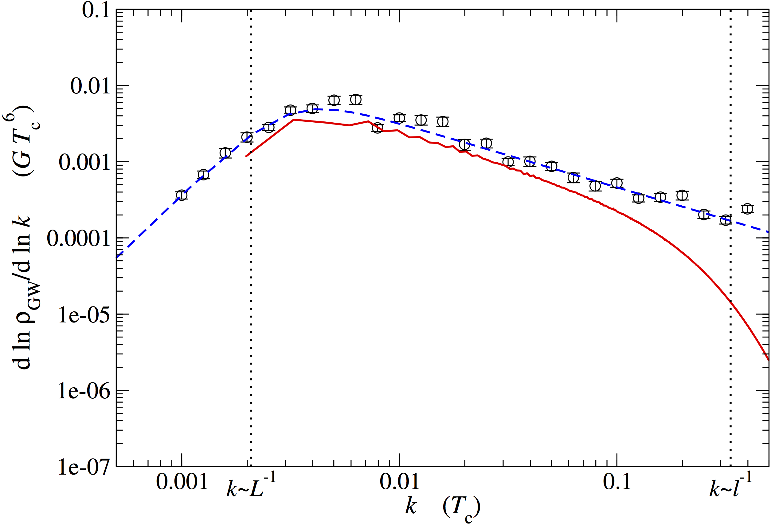
Envelope approximation: comparison with full scalar field simulations
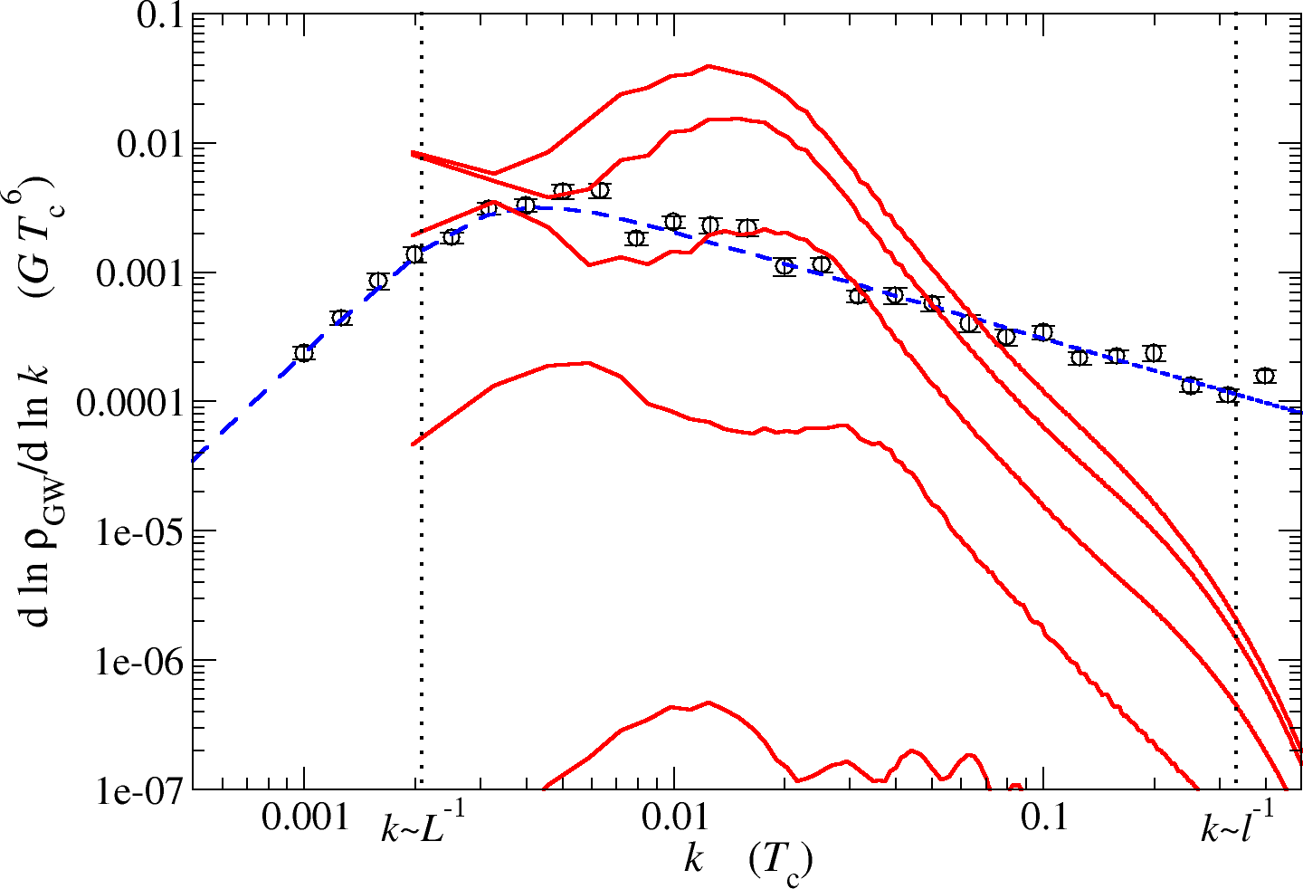
Envelope approximation: comparison with fluid source
Envelope approx.: recent developments
- The envelope approximation is a semi-numerical method which depends on multidimensional oscillatory integrals.
- It is difficult to implement accurately at high $f$, so the high-frequency power laws are not fully understood.
- In a recent paper, Jinno and Takimoto reproduced the results of the envelope approximation in a novel way
The calculation of Jinno and Takimoto
- Working in the same framework as the envelope approximation, further analytical progress
- Express the total power spectrum in terms of the
unequal time correlator $\langle T_{ij}(\mathbf{x},t_x)T_{lm}(\mathbf{y},t_y) \rangle $. The authors split it into two parts:
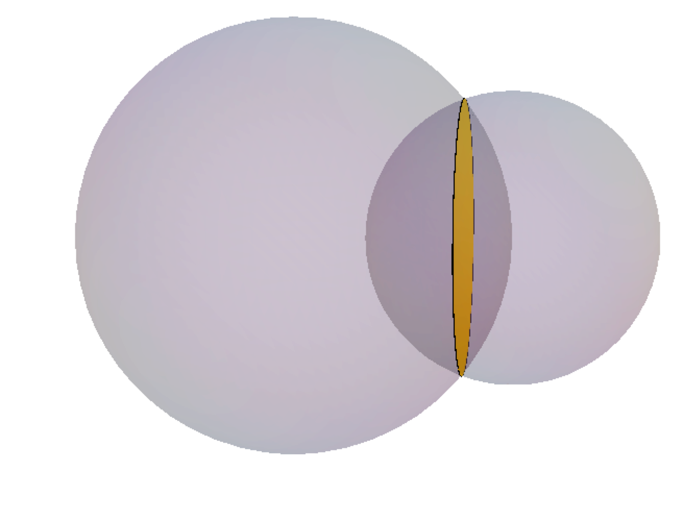
- A 'single-bubble' part, where the two points $\mathbf{x}$ and $\mathbf{y}$ lie on the surface of the same bubble.
- A 'double-bubble' parts, where they lie on two intersecting bubble walls.
- This allows the $k^{-1}$ high-power behaviour to be seen analytically by Taylor expanding the resulting correlator.
Jinno and Takimoto: results
Source: arXiv:1605.01403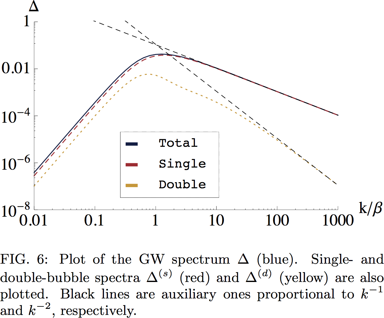
Two approximations: conclusion
- Quadrupole approximation totally overestimates result, because higher multipoles dominate
- Envelope approximation still incomplete for our purposes: it assumes source is a thin wall
- Most importantly, nothing we have seen so far considers what happens after the bubbles have collided
- In the next section, we will consider full simulations of the field-fluid model and see what results
6: Field-fluid simulations
Motivation
- Nothing else quite good enough:
- Quadrupole approximation is totally wrong
- Envelope approximation is an underestimate (sound shells thick, and dynamics after the collision)
- We already have a 'valid' model of the physics, consisting of a coupled scalar field $\phi$ and relativistic fluid $u^\mu$, so why not use that?
- Can easily measure gravitational waves by just solving the wave equation $$ \square h_{ij}^\text{TT} = 16 \pi G T_{ij}$$ numerically.
Further reading
- Spherical simulations of field-fluid model:
Kurki-Suonio and Laine hep-ph/9501216, hep-ph/9512202,
[+ Ignatius + Kajantie] astro-ph/9309059; Giblin and Mertens arXiv:1310.2948 - 3D simulations:
arXiv:1704.05871, arXiv:1504.03291, arXiv:1304.2433; Giblin and Mertens arXiv:1405.4005
Reminder: coupled field-fluid system
Ignatius, Kajantie, Kurki-Suonio and Laine- Scalar $\phi$ and ideal fluid $u^\mu$:
- Split stress-energy tensor $T^{\mu\nu}$ into field and fluid bits $$\partial_\mu T^{\mu\nu} = \partial_\mu (T^{\mu\nu}_\text{field} + T^{\mu\nu}_\text{fluid}) = 0$$
- Parameter $\eta$ sets the scale of friction due to plasma $$\partial_\mu T^{\mu\nu}_\text{field} = \tilde \eta \frac{\phi^2}{T} u^\mu \partial_\mu \phi \partial^\nu \phi \quad \partial_\mu T^{\mu\nu}_\text{fluid} = - \tilde \eta \frac{\phi^2}{T} u^\mu \partial_\mu \phi \partial^\nu \phi $$
- $V(\phi,T)$ is a 'toy' potential tuned to give latent heat $\mathcal{L}$
- $\beta$ ↔ number of bubbles; $\alpha_{T_*}$ ↔ $\mathcal{L}$, $v_\text{wall}$ ↔ $\tilde \eta$
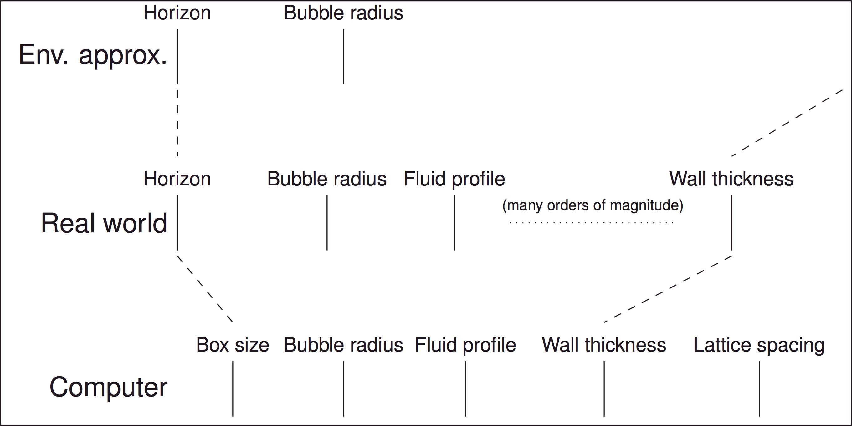
Dynamic range issues
- Most realtime lattice simulations in the early universe have a single [nontrivial] length scale
- Here, many length scales important
Implementation: Eulerian special relativistic hydrodynamics
Different things live in different places...
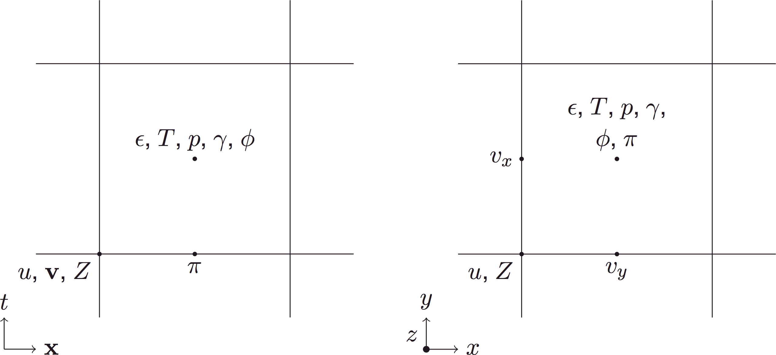
With this discretisation, evolution is second-order accurate!
Summary of algorithm 1:
- Original eom is: $$ (\partial_\mu \partial^\mu \phi) - \frac{\partial V_\text{eff}(\phi,T)}{\partial \phi} = -\eta(\phi, v_\mathrm{w}) u^\mu \partial_\mu \phi $$
- Use leapfrog + Crank-Nicolson algorithms for scalar field: \begin{align} \phi(x, t+\delta t) & = \phi(x,t) + \delta t \, \pi(x,t + \delta t/2) \\ \pi(x, t+\delta t/2) & = \frac{1}{1-z}\Bigg[(1+z)\pi(x, t-\delta t/2) + \delta t \bigg( \nabla^2 \phi(x, t) \\ & \qquad - \frac{\partial V_\text{eff}(\phi,T)}{\partial \phi} + \eta(\phi, v_\mathrm{w}) u^i \partial_i \phi(x,t) \bigg)\Bigg] \\ \end{align} where $z = - \delta t \, \eta(\phi, v_\mathrm{w}) \gamma $.
Summary of algorithm 2:
- Metric perturbations also evolved with leapfrog.
- Equation of motion is $$ - \ddot{h}_{ij}(x,t) +\nabla^2 h_{ij}(x,t) = 16 \pi G T^\text{source}_{ij}(x,t). $$ where the sources are $$ T^{\text{source},\,\phi}_{ij} = \partial_i \phi \partial_j \phi; \qquad T^{\text{source},\,\text{fluid}} = w u_i u _j $$
- This becomes $$ \begin{align} h_{ij}(x, t+\delta t) & = h_{ij}(x,t) + \delta t \, \dot{h}_{ij}(x,t+\delta t /2) \\ \dot h_{ij}(x, t+\delta t/2) & = \dot h_{ij}(x, t-\delta t/2) + \delta t\, \big[ \nabla^2 h_{ij}(x, t) \\ & \qquad + 16 \pi G T^\text{source}_{ij} (x, t) \big] \end{align}$$
Summary of algorithm 3:
- The fluid eom was $$ \partial_\mu (w u^\mu u^\nu) - \partial^\nu p + \frac{\partial V_\text{eff}(\phi,T)}{\partial \phi} \partial^\nu \phi = + \eta(\phi, v_\mathrm{w}) u^\mu \partial_\mu \phi \partial^\nu \phi $$
- Solving this accurately is rather more involved!
Operator splitting methods... Wilson and Matthews- Pressure acceleration
- Update velocities ($u_i$, $V_i$), gamma-factors
- Pressure work on fluid
- Advection of state variables
- Update velocities again
- Pressure work again
Velocity profile development: small $\tilde \eta$ ⇒ detonation (supersonic wall)
Velocity profile development: large $\tilde \eta$ ⇒ deflagration (subsonic wall)
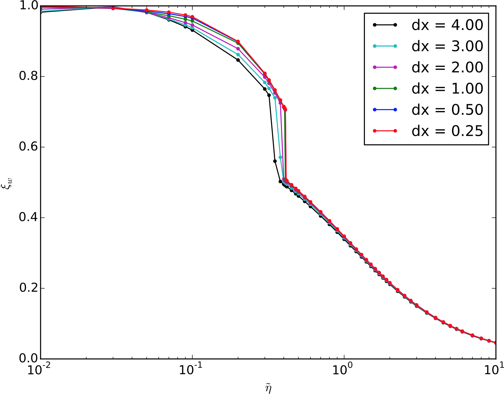
$v_\mathrm{w}$ as a function of $\tilde \eta$
Simulation slice example
Velocity power spectra and power laws
Fast deflagration
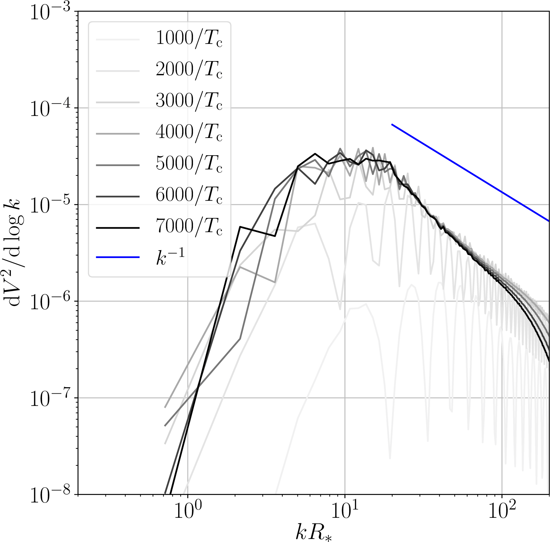
Detonation
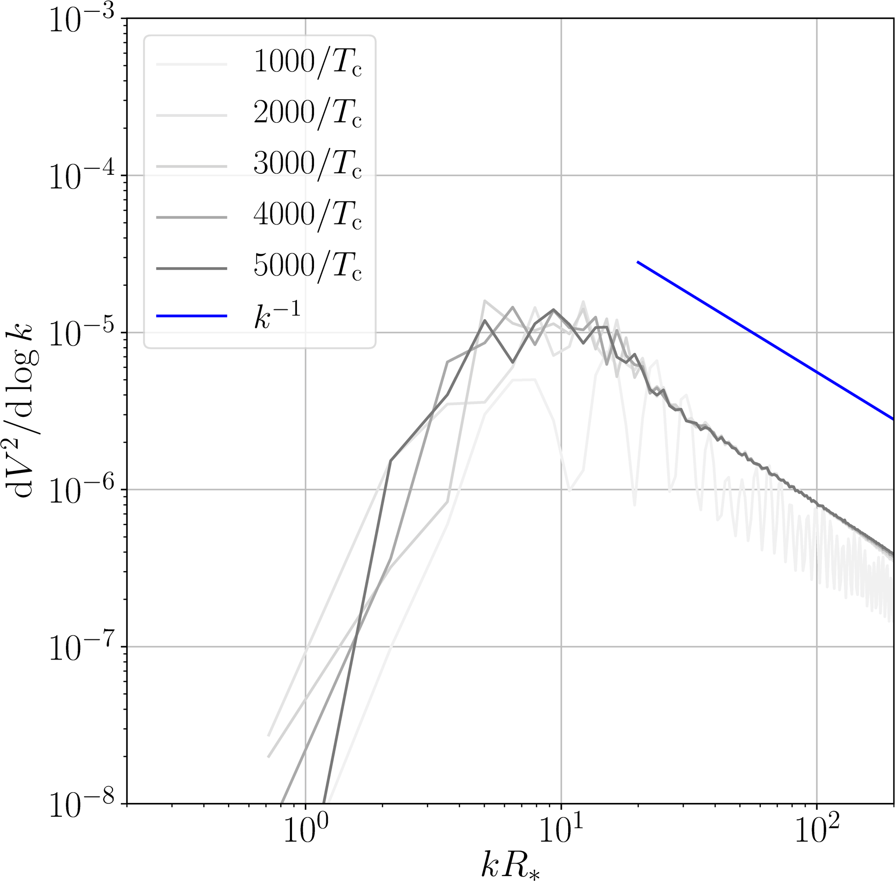
- Weak transition: $\alpha_{T_*} =0.01$
- Power law behaviour above peak is between $k^{-2}$ and $k^{-1}$
- “Ringing” due to simultaneous nucleation, unimportant
From $\phi$ and $u_\mu$ to $h_{ij}$ and $\Omega_\text{GW}$
- As discussed, simply evolve: $$ \square h_{ij}(x,t) = 16 \pi G T_{ij}^\text{source}(x,t). $$
- Note that when $T_{ij}^\text{source}(x,t) =
w(x)u_i(x)u_j(x)$ this is basically a convolution of the
fluid velocity power
(assuming $w(x) \approx \bar w$) Caprini, Durrer and Servant - When we want to measure the energy in gravitational waves, we do the projection to TT and measure: $$ t_{\mu\nu}^\text{GW}= \frac{1}{32 \pi G}\langle \partial_\mu h^\text{TT}_{ij} \partial_\nu h^\text{TT}_{ij} \rangle; \quad \rho_\text{GW} = \frac{1}{32 \pi G} \langle \dot{h}^\text{TT}_{ij} \dot{h}^\text{TT}_{ij} \rangle. $$
- We can then redshift this to present day to get $\Omega_\text{GW} h^2$.
Energy in gravitational waves
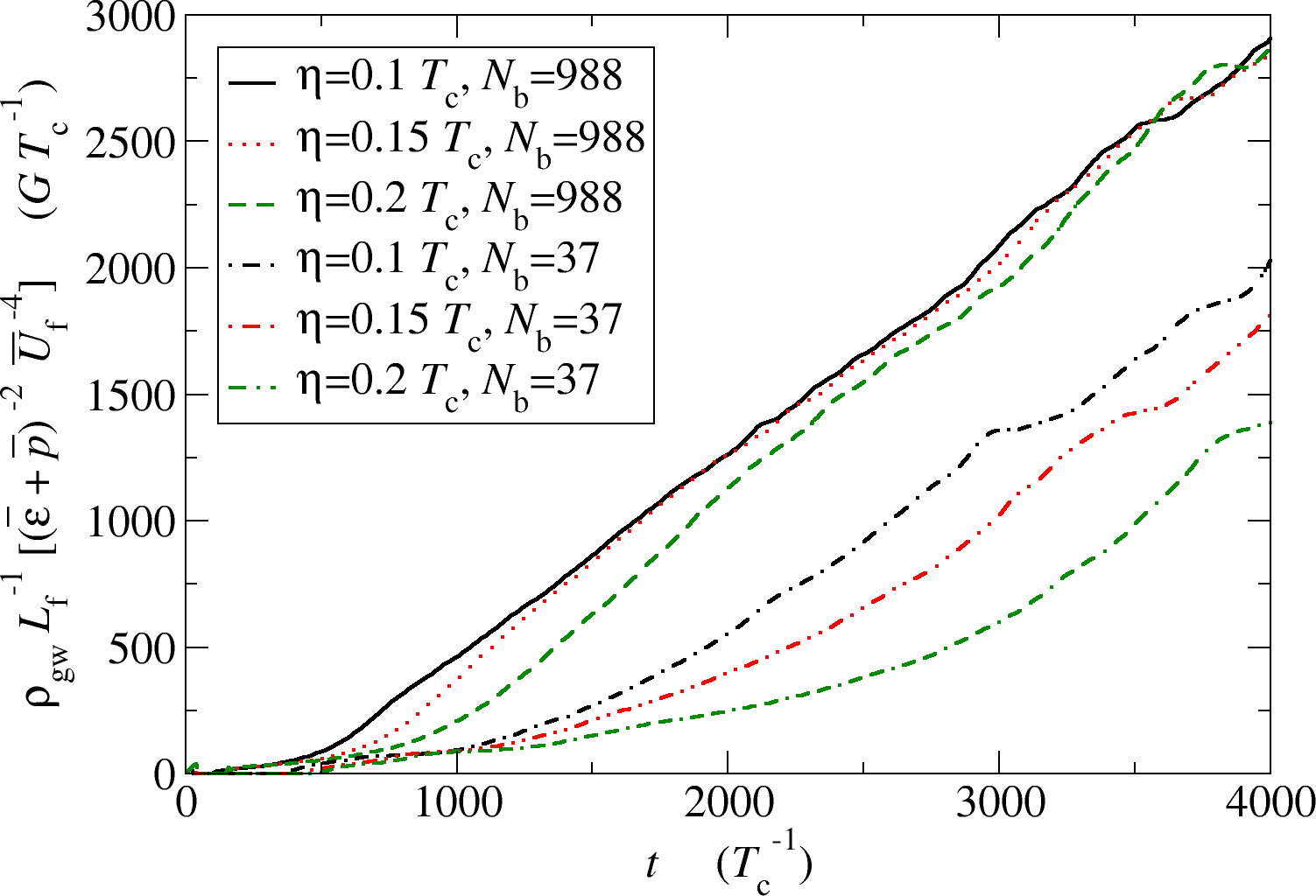
GW power spectra and power laws
Fast deflagration
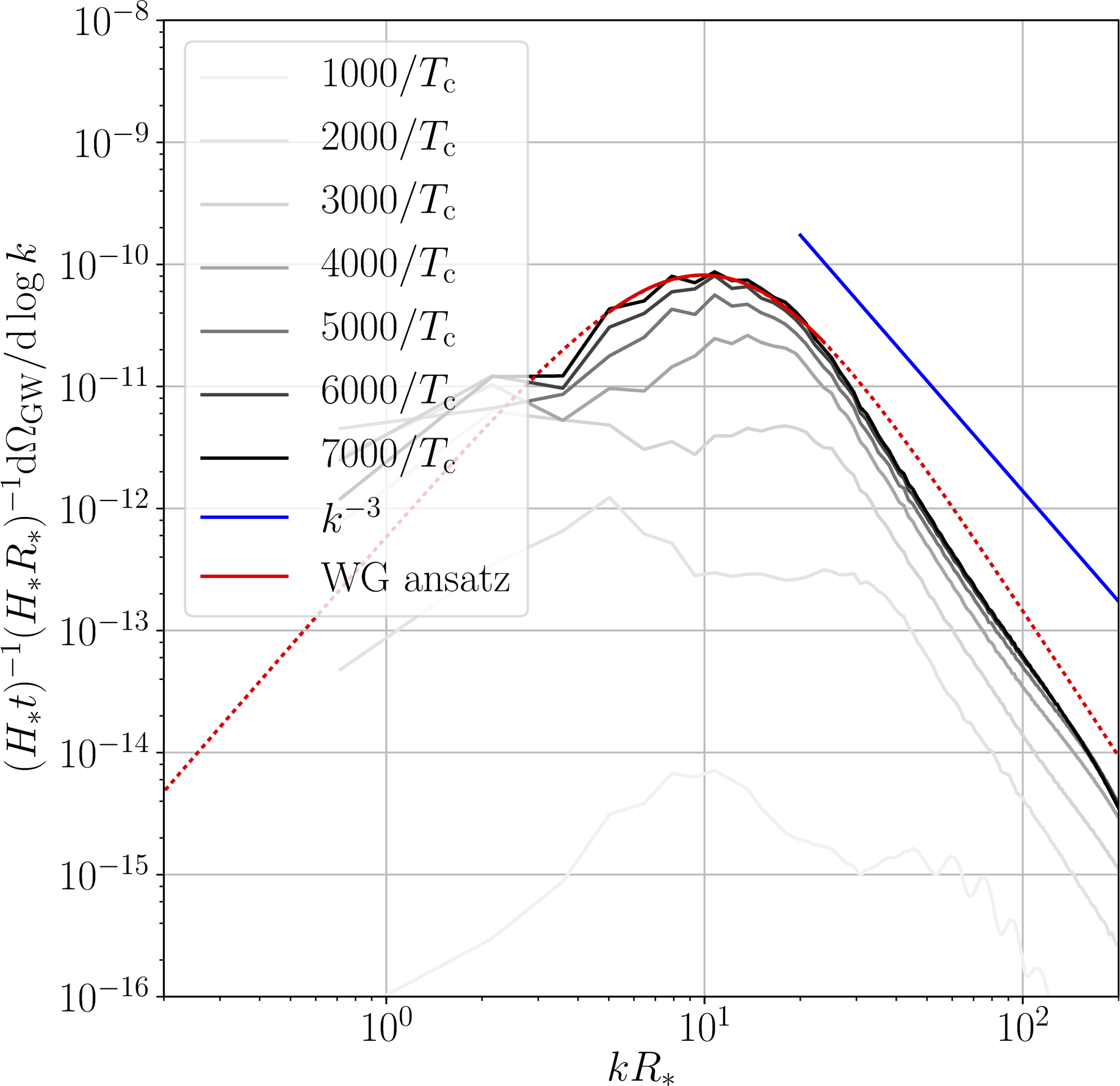
Detonation
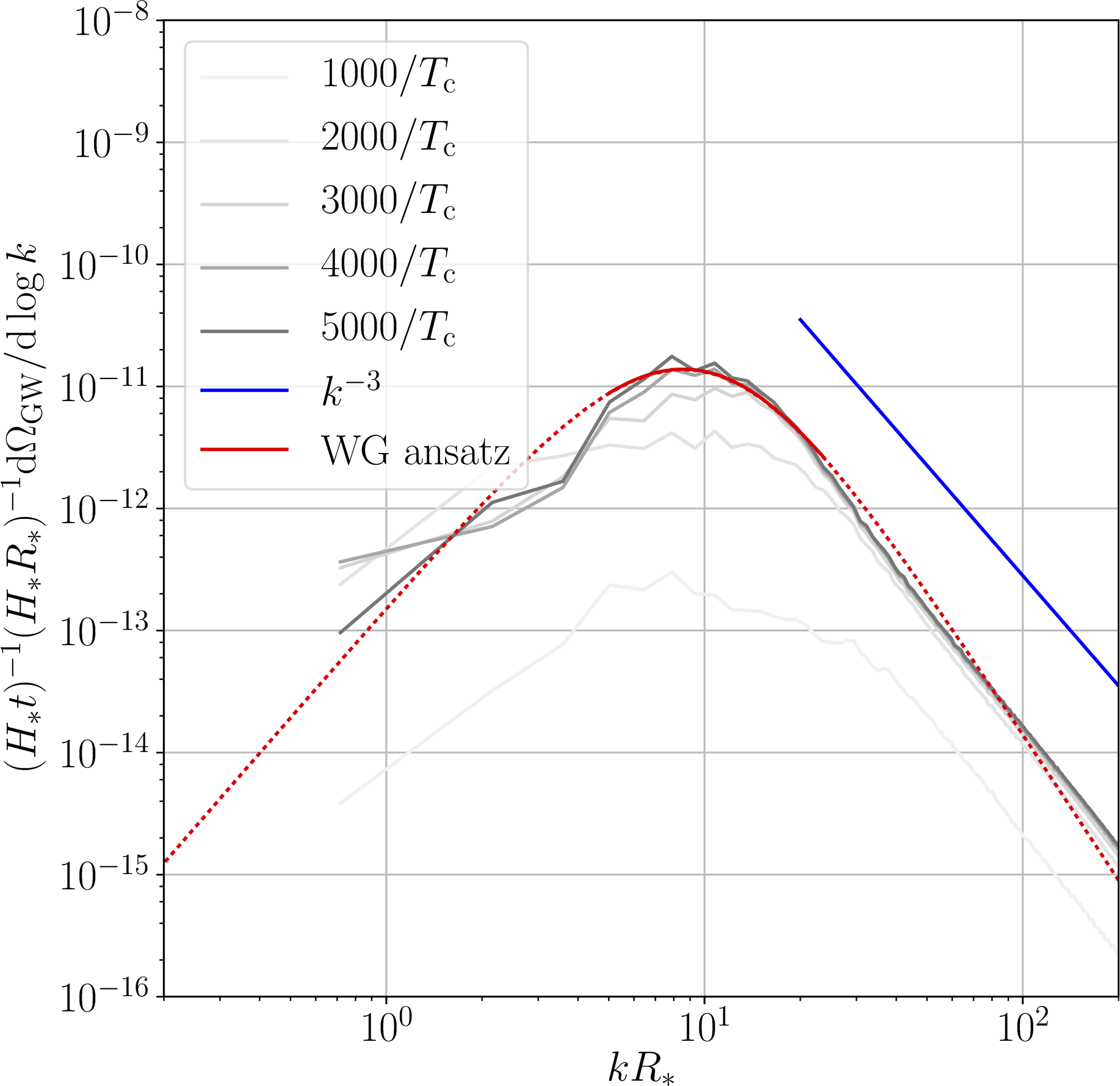
- Causal $k^3$ at low $k$, approximate $k^{-3}$ or $k^{-4}$ at high $k$
- Curves scaled by $t$: source until turbulence/expansion
A very important point:
- The acoustic source lasts a long time (about a Hubble time)
- It is also quite strong ($\kappa_\mathrm{f}\alpha$)
- It can therefore enhance the GW signal considerably!
⇒ more models detectable by LISA
Transverse versus longitudinal modes – turbulence?
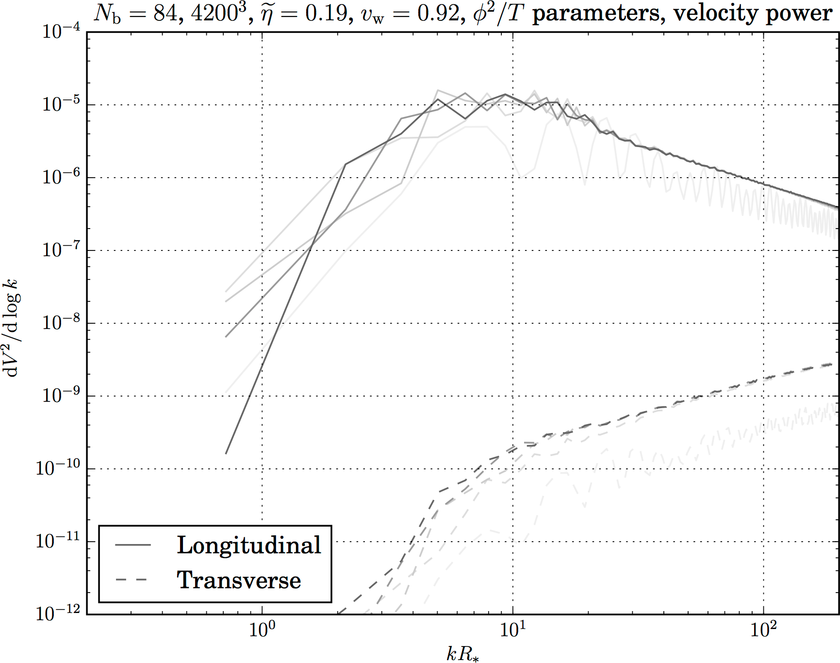
- Short simulation; weak transition (small $\alpha$): linear; most power in longitudinal modes ⇒ acoustic waves, turbulent
- Turbulence requires longer timescales $R_*/\overline{U}_\mathrm{f}$
- Plenty of theoretical results, use those instead
Kahniashvili et al.; Caprini, Durrer and Servant; Pen and Turok; ...
Simulations: conclusion
- Without solving the field theory equations of motion for everything (e.g. with hard thermal loops) or doing the Boltzmann equations, simulating the field-fluid model is the best we can do.
- Current cutting-edge simulations are still frustratingly small in size, need to extrapolate.
- Simulations too short to study turbulence.
- Therefore, use simulation results to derive ansätze and models, and combine with theoretical results where required to make predictions.
Models and predictions
Motivation
- For a given model - Higgs singlet, 2HDM, ... - compute the GW power spectrum.
- Approximately 4 inputs $\alpha$, $\beta$,
$v_\mathrm{w}$, $T_*$, all derivable from the
phenomenological model
- Perturbation theory (effective potential, etc.)
- Nonperturbative simulations
- Output: $\Omega_\text{gw} h^2$
- Then compare to LISA sensitivity curve (and others) and see if we could detect it
Further reading
- eLISA CosWG report: arXiv:1512.06239
Three sources
- We consider gravitational waves from three stages:
- Scalar field wall collisions: $\Omega_{\text{env}}$
- The acoustic regime: $\Omega_{\text{env}}$
- Turbulence: $\Omega_{\text{turb}}$
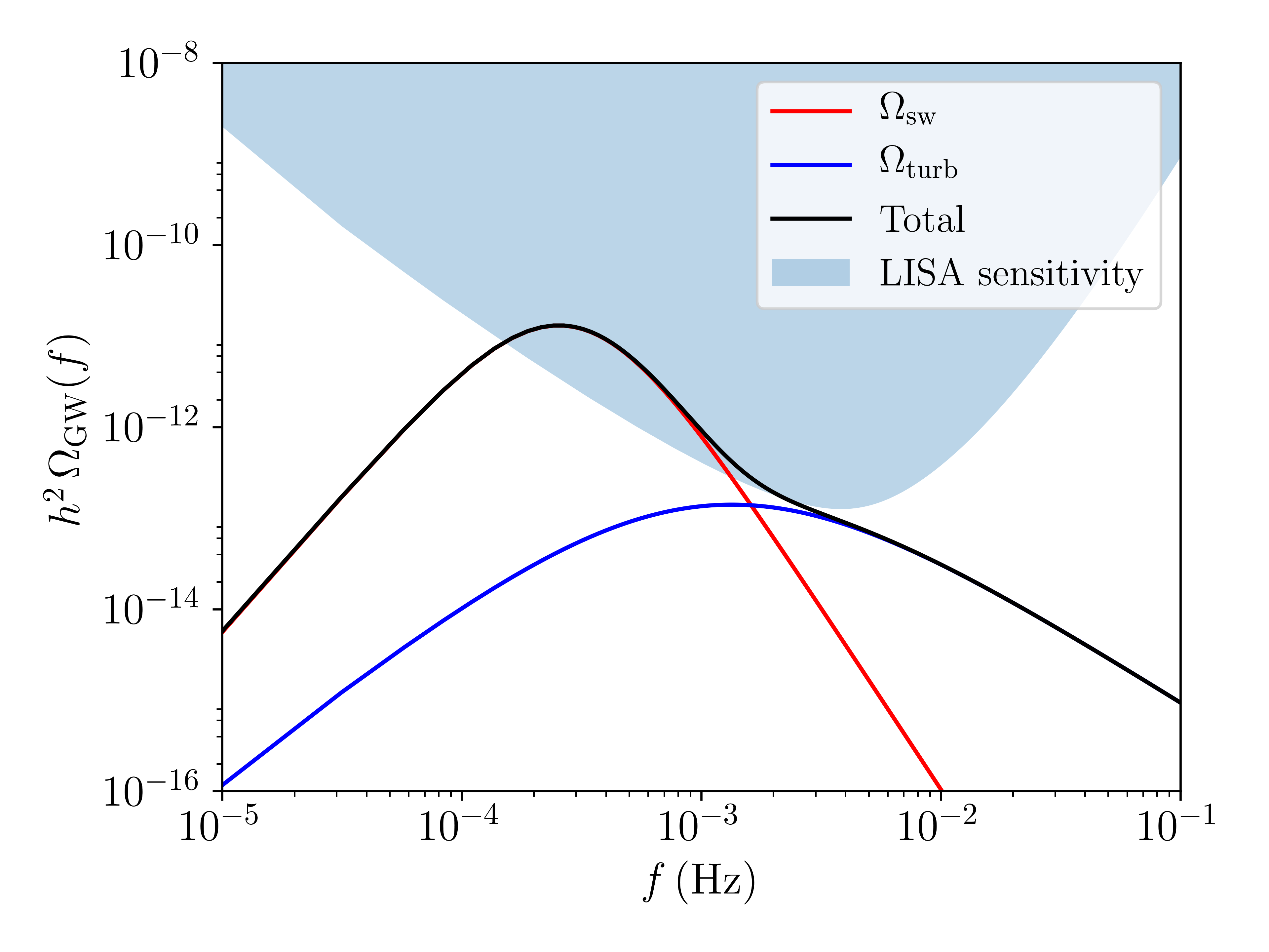
- They are expected to sum together: $$ \Omega_\text{GW} = \Omega_{\text{env}} + \Omega_{\text{sw}} + \Omega_{\text{turb}} $$
- Here we will consider ansätze for each in turn.
Colliding scalar fields: amplitude
arXiv:1605.01403- The amplitude is given by $ h^2 \Omega_\text{env}(f) = 1.67 \times 10^{-5} \, \Delta \left(\frac{H_*}{\beta}\right)^2 \left( \frac{\kappa_\phi \alpha_{T_*}}{1 + \alpha_{T_*}} \right)^2 \left(\frac{100}{g_*} \right)^{\frac{1}{3}} S_\text{env}(f) $
- The spectral shape is $ S_\text{env}(f) = \left[ c_l \left(\frac{f}{f_\text{env}}\right)^{-3} + (1 - c_l - c_h)\left(\frac{f}{f_\text{env}} \right)^{-1} + c_h \left(\frac{f}{f_\text{env}}\right) \right]^{-1} $ where $c_l = 0.064$ and $c_h = 0.48$.
- The wall velocity dependence is $\Delta = 0.48 v_\mathrm{w}^3/(1 + 5.3 v_\mathrm{w}^2 + 5 v_\mathrm{w}^4) $
Colliding scalar fields: frequency
arXiv:1605.01403- The peak frequency in the spectral shape is given by $$ f_\text{env} = 16.5 \, \mu\mathrm{Hz} \, \left(\frac{f_*}{\beta} \right) \left( \frac{\beta}{H_*} \right) \left( \frac{T_*}{100 \, \mathrm{GeV}} \right) \left( \frac{g_*}{100} \right)^{\frac{1}{6}} $$
- The wall velocity dependence of $f_\text{env}$ is $$\frac{f_*}{\beta} = \frac{0.35}{1 + 0.069 v_\mathrm{w} + 0.69 v_\mathrm{w}^4}. $$
Acoustic waves: amplitude
arXiv:1704.05871- The amplitude is given by $$h^2 \Omega_\text{sw}(f) = 8.5 \times 10^{-6} \left(\frac{100}{g_*} \right)^{\frac{1}{3}} \Gamma^2 \overline{U}_\mathrm{f}^4 \left(\frac{H}{\beta}\right) v_\mathrm{w} \, S_\text{sw}(f)$$ where $\Gamma = \overline{w}/\overline{\epsilon} \approx 4/3$; $\overline{w}$ and $\overline{\epsilon}$ are the volume-averaged enthalpy and energy density
- $\overline{U}_\mathrm{f}$ is a measure of the rms fluid velocity $$\overline{U}_\mathrm{f}^2 = \frac{1}{\overline w} \frac{1}{\mathcal{V}} \int_\mathcal{V} d^3 x \, \tau_{ii}^\mathrm{f} \approx \frac{3}{4} \kappa_\mathrm{f} \alpha_{T_*}$$
Acoustic waves: frequency
arXiv:1704.05871- The spectral shape is $$ S_\text{sw}(f) = \left(\frac{f}{f_\mathrm{sw}}\right)^3 \left( \frac{7}{4 + 3 (f/f_\mathrm{sw})^2 } \right)^{7/2}$$
- The approximate peak frequency is $$ f_\mathrm{sw} = 8.9 \, \mu\mathrm{Hz} \, \frac{1}{v_\mathrm{w}} \left( \frac{\beta}{H_*} \right) \left( \frac{z_\mathrm{p}}{10} \right) \left( \frac{T_*}{100 \, \mathrm{GeV}}\right) \left( \frac{g_*}{100} \right)^\frac{1}{6} $$
- Here $z_\mathrm{p}$ is a simulation-derived factor that is usually around 10
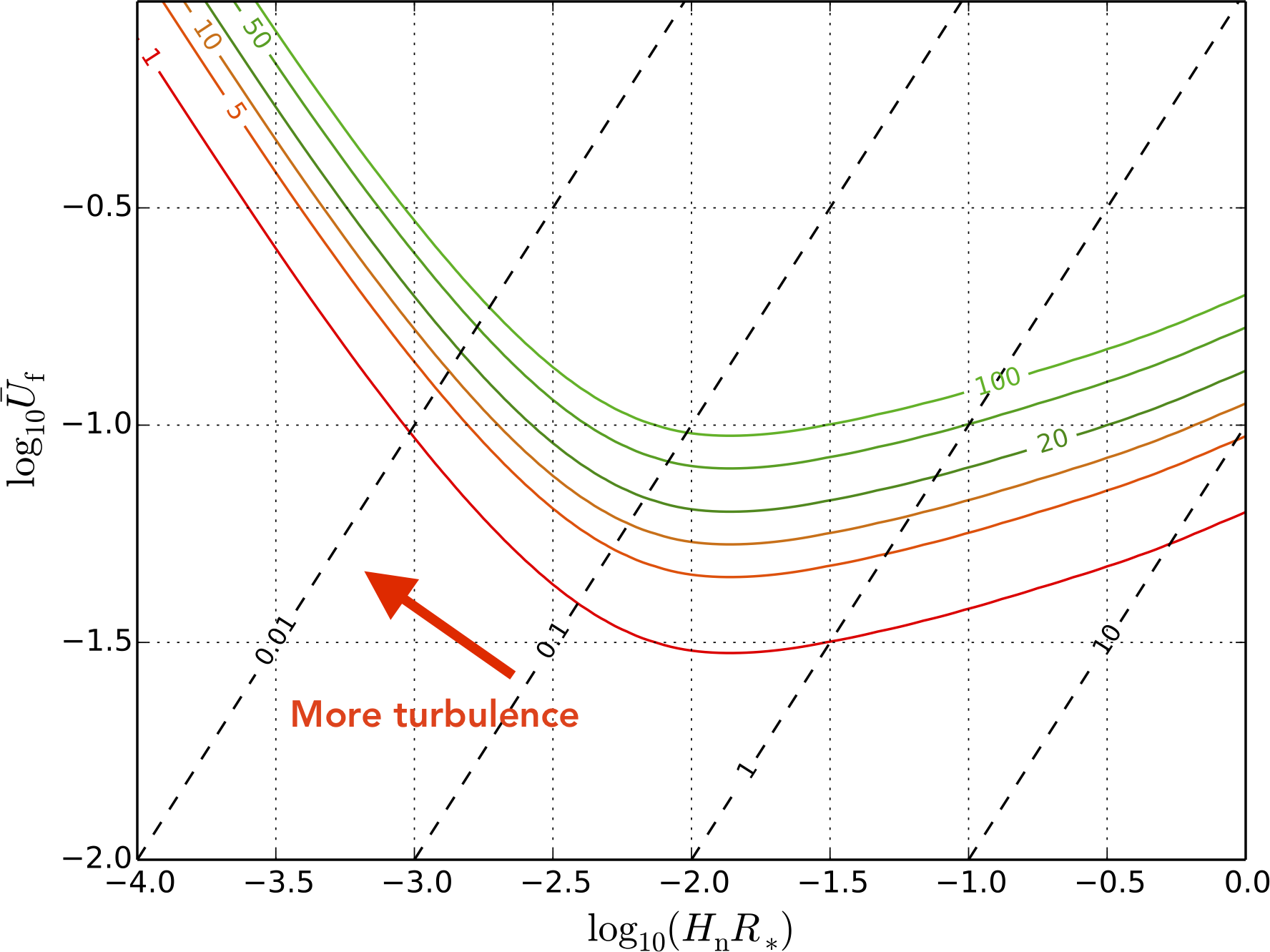
Detectability from acoustic waves alone
arXiv:1704.05871- In many cases, sound waves dominant
- Parametrise by RMS fluid velocity $\overline{U}_\mathrm{f}$ and bubble radius $R_*$
Turbulence: amplitude
- While the colliding scalar shells and acoustic wave sources are based on simulation results, here we resort to the analytical literature.
- Kolmogorov-type turbulence yields $ h^2 \Omega_\text{turb} (f) = 3.35 \times 10^{-4} \left( \frac{H_*}{\beta} \right) \left( \frac{\kappa_\text{turb} \alpha_{T_*}}{1 + \alpha_{T_*}} \right)^{\frac{3}{2}} \left( \frac{100}{g_*} \right)^{\frac{1}{3}} v_\mathrm{w} S_\text{turb}(f) $
- Here $\kappa_\text{turb}$ is the efficiency of conversion of latent heat into turbulent flows. On short timescales it is very small (a few percent at most).
- Shocks and turbulence develop on timescale: $ \tau_\text{sh} \sim \mathrm{L}_f / \overline{U}_\mathrm{f}. $
Turbulence: spectral shape
- Although the amplitude is uncertain and will have to wait for future simulations, the peak frequency is known exactly, $$ S_\text{turb}(f) = \frac{(f/f_\text{turb})^3}{[1+(f/f_\text{turb})]^{\frac{11}{3}}} ( 1 + 8 \pi f/h_*). $$
- Here $h_*$ is the Hubble rate at $T_*$: $$ h_* = 16.5 \, \mu\mathrm{Hz} \left( \frac{T_*}{100 \, \mathrm{GeV} }\right) \left(\frac{g_*}{100} \right)^{\frac{1}{6}}$$
Turbulence: peak frequency
- The peak frequency $f_\text{turb}$ is slightly higher than for the sound wave contribution, $$ f_\text{turb} = 27 \, \mu\mathrm{Hz} \, \frac{1}{v_\mathrm{w}} \left( \frac{\beta}{H_*} \right) \left(\frac{T_*}{100 \, \mathrm{GeV}} \right) \left(\frac{g_*}{100}\right)^{\frac{1}{6}}. $$
From a model to a GW power spectrum
Here, $\alpha = 0.084$, $v_\mathrm{w} = 0.44$, $T_* = 180 \, \mathrm{GeV}$ and $\beta/H_* = 10$
Final conclusion
- The electroweak phase transition is 'wide open':
- The LHC cannot rule out some very interesting scenarios
- Baryogenesis, dark matter, GWs, ...
- We have an excellent understanding of first-order thermal phase transitions, from the bottom up.
- We can now make pretty confident estimates of the gravitational wave power spectrum.
- Recently appreciated contributions, like the acoustic waves, help to enhance the source considerably.
A pipeline?
- Choose your model
(e.g. SM, xSM, 2HDM, ...) - Dim. red. model Kajantie et al.
- Phase diagram ($\alpha_{T_*}$, $T_*$);
lattice: Kajantie et al. - Nucleation rate ($\beta$);
lattice: Moore and Rummukainen - Wall velocities ($v_\text{wall}$)
Moore and Prokopec; Kozaczuk - GW power spectrum $\Omega_\mathrm{gw}$
- Sphaleron rate
Very leaky, even for SM!
Thank you!
- I hope you have enjoyed these lectures as much as I have enjoyed preparing and presenting them.
- If you have any questions, comments, or feedback,
please get in touch!