CosWG - PTPlot
David Weir
Demo

Fluid source
$$ \frac{d \Omega_{\text{gw},0}}{d \ln(f)} = 0.68 F_{\text{gw},0} \Gamma^2 \overline{U}^4_\text{f} (H_n R_*) \tilde{\Omega}_\text{gw} C\left(\frac{f}{f_{\text{p},0}}\right), $$
where
0.68 is $2/(8\pi)^{1/3}$
😅
Fluid source
$$ \frac{d \Omega_{\text{gw},0}}{d \ln(f)} = 0.68 F_{\text{gw},0} \Gamma^2 \overline{U}^4_\text{f} (H_n R_*) \tilde{\Omega}_\text{gw} C\left(\frac{f}{f_{\text{p},0}}\right), $$
where
$$ F_{\text{gw},0} = (3.57 \pm 0.05)\times 10^{-5} \left(\frac{100}{g_*}\right)^{\frac{1}{3}} $$
(redshifting)
Fluid source
$$ \frac{d \Omega_{\text{gw},0}}{d \ln(f)} = 0.68 F_{\text{gw},0} \Gamma^2 \overline{U}^4_\text{f} (H_n R_*) \tilde{\Omega}_\text{gw} C\left(\frac{f}{f_{\text{p},0}}\right), $$
where
$\Gamma = 1 + \frac{\large \overline{p}}{\large \overline{\varepsilon}} \approx \frac{4}{3}$
(adiabatic index)
Fluid source
$$ \frac{d \Omega_{\text{gw},0}}{d \ln(f)} = 0.68 F_{\text{gw},0} \Gamma^2 \overline{U}^4_\text{f} (H_n R_*) \tilde{\Omega}_\text{gw} C\left(\frac{f}{f_{\text{p},0}}\right), $$
where
$$ \overline{U}^2_\text{f} = \frac{1}{(\overline{p} + \overline{\varepsilon}) V}\int_{V} d^3 x \, \tau^{\mathrm{(f)}}_{ii} = f(\alpha, v_\mathrm{w})$$
(fluid kinetic energy)
What is $f(\alpha, v_\mathrm{w})$?
$$\overline{U}_\mathrm{f}^2 = \frac{3}{4} \alpha\, \kappa_\mathrm{v}(v_\mathrm{w},\alpha)$$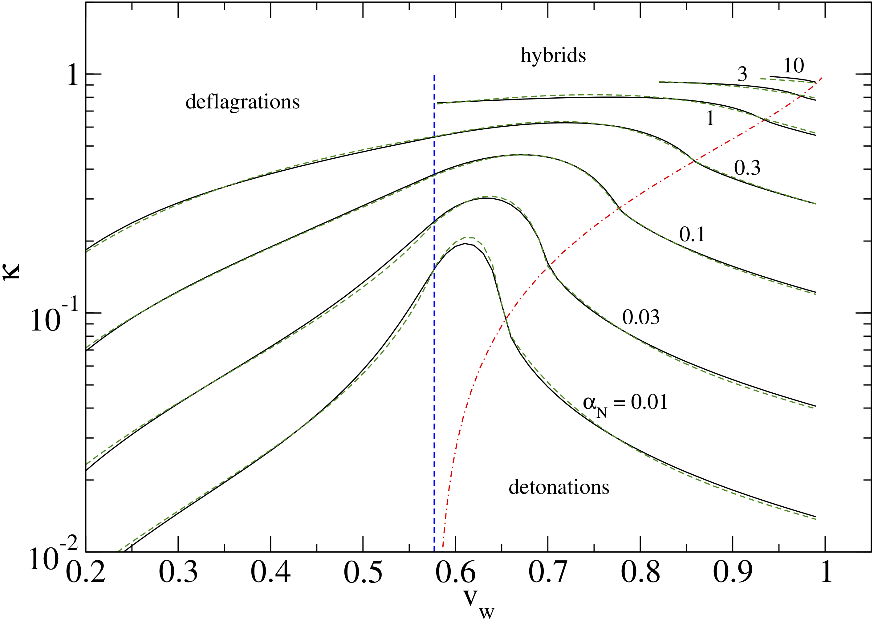
Fluid source
$$ \frac{d \Omega_{\text{gw},0}}{d \ln(f)} = 0.68 F_{\text{gw},0} \Gamma^2 \overline{U}^4_\text{f} (H_n R_*) \tilde{\Omega}_\text{gw} C\left(\frac{f}{f_{\text{p},0}}\right), $$
where
$$ \tilde{\Omega}_\text{gw} \approx 0.12 $$
(universal amplitude fitted from simulations)
Fluid source
$$ \frac{d \Omega_{\text{gw},0}}{d \ln(f)} = 0.68 F_{\text{gw},0} \Gamma^2 \overline{U}^4_\text{f} (H_n R_*) \tilde{\Omega}_\text{gw} C\left(\frac{f}{f_{\text{p},0}}\right), $$
where
$$ C(s) = s^3\left(\frac{7}{4+3s^2}\right)^{7/2} $$
(spectral shape supported by latest simulations)
Fluid source
$$ \frac{d \Omega_{\text{gw},0}}{d \ln(f)} = 0.68 F_{\text{gw},0} \Gamma^2 \overline{U}^4_\text{f} (H_n R_*) \tilde{\Omega}_\text{gw} C\left(\frac{f}{f_{\text{p},0}}\right), $$
where
$$ f_{\text{p},0} \simeq 26 \left( \frac{1}{H_\mathrm{n}R_*} \right) \left( \frac{z_\mathrm{p}}{10} \right) \left( \frac{T_\mathrm{n}}{10^2 \, \text{GeV}} \right) \left( \frac{g_*}{100} \right)^{\frac{1}{6}} \; \mu\text{Hz} $$
(peak frequency)
Peak frequency
$$ f_{\text{p},0} \simeq 26 \left( \frac{1}{H_\mathrm{n}R_*} \right) \left( \frac{z_\mathrm{p}}{10} \right) \left( \frac{T_\mathrm{n}}{10^2 \, \text{GeV}} \right) \left( \frac{g_*}{100} \right)^{\frac{1}{6}} \; \mu\text{Hz} $$
where
$z_\mathrm{p}$ is the peak $k R_* \approx 10$ (weak function of $v_\mathrm{w}$, ...)
Online tool?
- Web-based, open to all (mostly?)
- Power spectra and SNR plots
- Output vector graphics (SVG)
- ... but not slow to run
- ... securely containerised
Features
- Python (w/ Django framework)
- Matplotlib
- Git repo, collaborators welcome
- Source code available
- Can also be run standalone